PYTORCH 卷积神经网络+CIFAR10数据分类+用VGG16对CIFAR10分类（代码练习）

一、卷积神经网

import torch
import torch.nn as nn
import torch.nn.functional as F
import torch.optim as optim
from torchvision import datasets, transforms
import matplotlib.pyplot as plt
import numpy

# 一个函数，用来计算模型中有多少参数
def get_n_params(model):
    np=0
    for p in list(model.parameters()):
        np += p.nelement()
    return np

# 使用GPU训练，可以在菜单 "代码执行工具" -> "更改运行时类型" 里进行设置
device = torch.device("cuda:0" if torch.cuda.is_available() else "cpu")

深度神经网络特性：

• 很多层: compositionality
• 卷积: locality + stationarity of images
• 池化: Invariance of object class to translations

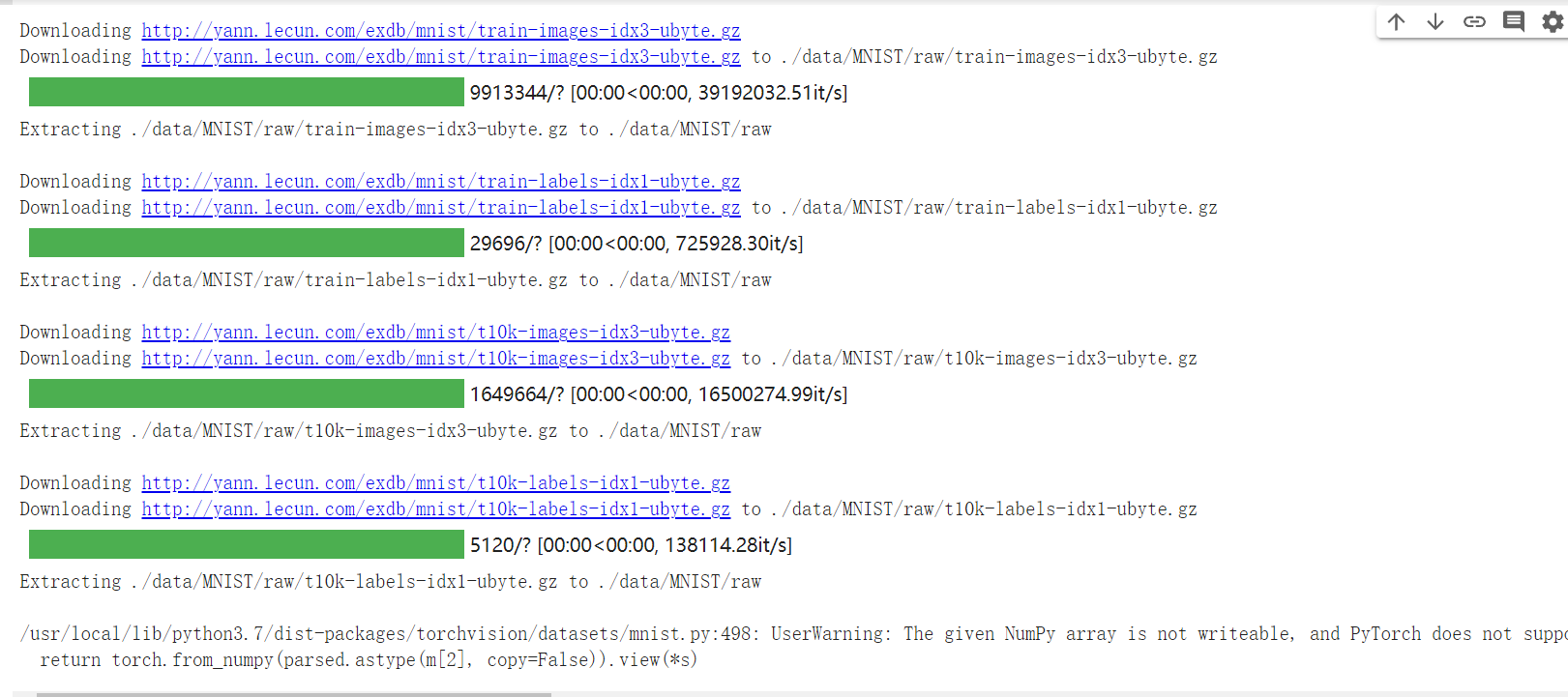
1.加载数据（MNIST)

input_size  = 28*28   # MNIST上的图像尺寸是 28x28
output_size = 10      # 类别为 0 到 9 的数字，因此为十类

train_loader = torch.utils.data.DataLoader(
    datasets.MNIST('./data', train=True, download=True,
        transform=transforms.Compose(
            [transforms.ToTensor(),
             transforms.Normalize((0.1307,), (0.3081,))])),
    batch_size=64, shuffle=True)

test_loader = torch.utils.data.DataLoader(
    datasets.MNIST('./data', train=False, transform=transforms.Compose([
             transforms.ToTensor(),
             transforms.Normalize((0.1307,), (0.3081,))])),
    batch_size=1000, shuffle=True)

 显示数据集中的部分图像

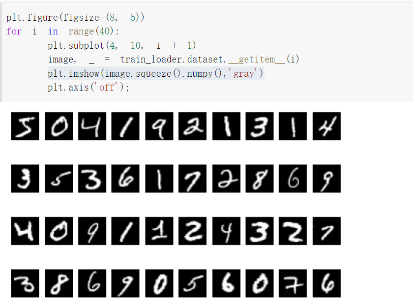
plt.figure(figsize=(8, 5))表示figure的长、宽（单位inch）

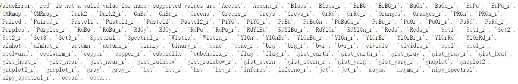
plt.imshow(image.squeeze().numpy(),'gray')gray取灰度图。

2.创建网络

定义网络时，需要继承nn.Module，并实现它的forward方法，把网络中具有可学习参数的层放在构造函数init中。

只要在nn.Module的子类中定义了forward函数，backward函数就会自动被实现(利用autograd)。

class FC2Layer(nn.Module):
    def __init__(self, input_size, n_hidden, output_size):
        # nn.Module子类的函数必须在构造函数中执行父类的构造函数
        # 下式等价于nn.Module.__init__(self)        
        super(FC2Layer, self).__init__()
        self.input_size = input_size
        # 这里直接用 Sequential 就定义了网络，注意要和下面 CNN 的代码区分开
        self.network = nn.Sequential(
            nn.Linear(input_size, n_hidden), 
            nn.ReLU(), 
            nn.Linear(n_hidden, n_hidden), 
            nn.ReLU(), 
            nn.Linear(n_hidden, output_size), 
            nn.LogSoftmax(dim=1)
        )
    def forward(self, x):
        # view一般出现在model类的forward函数中，用于改变输入或输出的形状
        # x.view(-1, self.input_size) 的意思是多维的数据展成二维
        # 代码指定二维数据的列数为 input_size=784，行数 -1 表示我们不想算，电脑会自己计算对应的数字
        # 在 DataLoader 部分，我们可以看到 batch_size 是64，所以得到 x 的行数是64
        # 大家可以加一行代码：print(x.cpu().numpy().shape)
        # 训练过程中，就会看到 (64, 784) 的输出，和我们的预期是一致的

        # forward 函数的作用是，指定网络的运行过程，这个全连接网络可能看不啥意义，
        # 下面的CNN网络可以看出 forward 的作用。
        x = x.view(-1, self.input_size)
        return self.network(x)
    


class CNN(nn.Module):
    def __init__(self, input_size, n_feature, output_size):
        # 执行父类的构造函数，所有的网络都要这么写
        super(CNN, self).__init__()
        # 下面是网络里典型结构的一些定义，一般就是卷积和全连接
        # 池化、ReLU一类的不用在这里定义
        self.n_feature = n_feature
        self.conv1 = nn.Conv2d(in_channels=1, out_channels=n_feature, kernel_size=5)
        self.conv2 = nn.Conv2d(n_feature, n_feature, kernel_size=5)
        self.fc1 = nn.Linear(n_feature*4*4, 50)
        self.fc2 = nn.Linear(50, 10)    
    
    # 下面的 forward 函数，定义了网络的结构，按照一定顺序，把上面构建的一些结构组织起来
    # 意思就是，conv1, conv2 等等的，可以多次重用
    def forward(self, x, verbose=False):
        x = self.conv1(x)
        x = F.relu(x)
        x = F.max_pool2d(x, kernel_size=2)
        x = self.conv2(x)
        x = F.relu(x)
        x = F.max_pool2d(x, kernel_size=2)
        x = x.view(-1, self.n_feature*4*4)
        x = self.fc1(x)
        x = F.relu(x)
        x = self.fc2(x)
        x = F.log_softmax(x, dim=1)
        return x

def train(model):
    model.train()
    # 主里从train_loader里，64个样本一个batch为单位提取样本进行训练
    for batch_idx, (data, target) in enumerate(train_loader):
        # 把数据送到GPU中
        data, target = data.to(device), target.to(device)

        optimizer.zero_grad()
        output = model(data)
        loss = F.nll_loss(output, target)
        loss.backward()
        optimizer.step()
        if batch_idx % 100 == 0:
            print('Train: [{}/{} ({:.0f}%)]\tLoss: {:.6f}'.format(
                batch_idx * len(data), len(train_loader.dataset),
                100. * batch_idx / len(train_loader), loss.item()))


def test(model):
    model.eval()
    test_loss = 0
    correct = 0
    for data, target in test_loader:
        # 把数据送到GPU中
        data, target = data.to(device), target.to(device)
        # 把数据送入模型，得到预测结果
        output = model(data)
        # 计算本次batch的损失，并加到 test_loss 中
        test_loss += F.nll_loss(output, target, reduction='sum').item()
        # get the index of the max log-probability，最后一层输出10个数，
        # 值最大的那个即对应着分类结果，然后把分类结果保存在 pred 里
        pred = output.data.max(1, keepdim=True)[1]
        # 将 pred 与 target 相比，得到正确预测结果的数量，并加到 correct 中
        # 这里需要注意一下 view_as ，意思是把 target 变成维度和 pred 一样的意思                                                
        correct += pred.eq(target.data.view_as(pred)).cpu().sum().item()

    test_loss /= len(test_loader.dataset)
    accuracy = 100. * correct / len(test_loader.dataset)
    print('\nTest set: Average loss: {:.4f}, Accuracy: {}/{} ({:.0f}%)\n'.format(
        test_loss, correct, len(test_loader.dataset),
        accuracy))

 　　

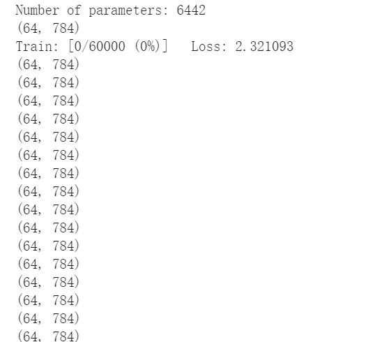
加入print(x.cpu().numpy().shape)出现（64，784）

去掉print(x.cpu().numpy().shape)后

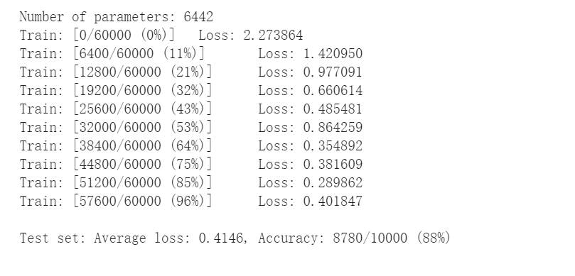
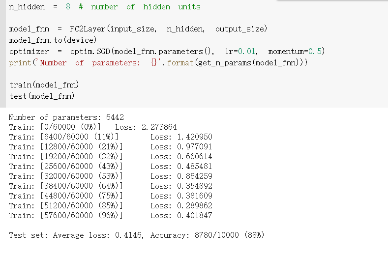
3.在小型全连接网络上训练（Fully-connected network）

 4.在卷积神经网络上训练

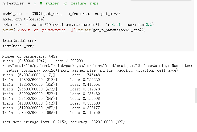
 通过上面的测试结果发现，含有相同参数的 CNN 效果要明显优于简单的全连接网络，是因为 CNN 能够通过卷积和池化更好的挖掘图像中的信息

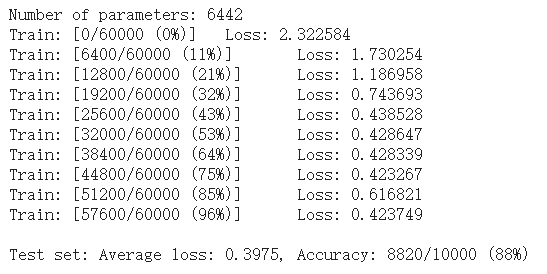
5. 打乱像素顺序再次在两个网络上训练与测试

下面代码展示随机打乱像素顺序后，图像的形态：

# 这里解释一下 torch.randperm 函数，给定参数n，返回一个从0到n-1的随机整数排列
perm = torch.randperm(784)
plt.figure(figsize=(8, 4))
for i in range(10):
    image, _ = train_loader.dataset.__getitem__(i)
    # permute pixels
    image_perm = image.view(-1, 28*28).clone()
    image_perm = image_perm[:, perm]
    image_perm = image_perm.view(-1, 1, 28, 28)
    plt.subplot(4, 5, i + 1)
    plt.imshow(image.squeeze().numpy(), 'gray')
    plt.axis('off')
    plt.subplot(4, 5, i + 11)
    plt.imshow(image_perm.squeeze().numpy(), 'gray')
    plt.axis('off')

# 对每个 batch 里的数据，打乱像素顺序的函数
def perm_pixel(data, perm):
    # 转化为二维矩阵
    data_new = data.view(-1, 28*28)
    # 打乱像素顺序
    data_new = data_new[:, perm]
    # 恢复为原来4维的 tensor
    data_new = data_new.view(-1, 1, 28, 28)
    return data_new

# 训练函数
def train_perm(model, perm):
    model.train()
    for batch_idx, (data, target) in enumerate(train_loader):
        data, target = data.to(device), target.to(device)
        # 像素打乱顺序
        data = perm_pixel(data, perm)

        optimizer.zero_grad()
        output = model(data)
        loss = F.nll_loss(output, target)
        loss.backward()
        optimizer.step()
        if batch_idx % 100 == 0:
            print('Train: [{}/{} ({:.0f}%)]\tLoss: {:.6f}'.format(
                batch_idx * len(data), len(train_loader.dataset),
                100. * batch_idx / len(train_loader), loss.item()))

# 测试函数
def test_perm(model, perm):
    model.eval()
    test_loss = 0
    correct = 0
    for data, target in test_loader:
        data, target = data.to(device), target.to(device)

        # 像素打乱顺序
        data = perm_pixel(data, perm)

        output = model(data)
        test_loss += F.nll_loss(output, target, reduction='sum').item()
        pred = output.data.max(1, keepdim=True)[1]                                            
        correct += pred.eq(target.data.view_as(pred)).cpu().sum().item()

    test_loss /= len(test_loader.dataset)
    accuracy = 100. * correct / len(test_loader.dataset)
    print('\nTest set: Average loss: {:.4f}, Accuracy: {}/{} ({:.0f}%)\n'.format(
        test_loss, correct, len(test_loader.dataset),
        accuracy))

perm = torch.randperm(784)
n_hidden = 8 # number of hidden units

model_fnn = FC2Layer(input_size, n_hidden, output_size)
model_fnn.to(device)
optimizer = optim.SGD(model_fnn.parameters(), lr=0.01, momentum=0.5)
print('Number of parameters: {}'.format(get_n_params(model_fnn)))

train_perm(model_fnn, perm)
test_perm(model_fnn, perm)

perm = torch.randperm(784)
n_features = 6 # number of feature maps

model_cnn = CNN(input_size, n_features, output_size)
model_cnn.to(device)
optimizer = optim.SGD(model_cnn.parameters(), lr=0.01, momentum=0.5)
print('Number of parameters: {}'.format(get_n_params(model_cnn)))

train_perm(model_cnn, perm)
test_perm(model_cnn, perm)

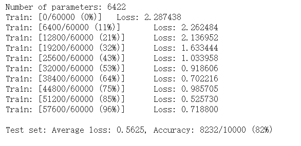
从打乱像素顺序的实验结果来看，全连接网络的性能基本上没有发生变化，但是 卷积神经网络的性能明显下降。

这是因为对于卷积神经网络，会利用像素的局部关系，但是打乱顺序以后，这些像素间的关系将无法得到利用。

二、CIFAR10数据分类

input[channel] = (input[channel] - mean[channel]) / std[channel]

import torch
import torchvision
import torchvision.transforms as transforms
import matplotlib.pyplot as plt
import numpy as np
import torch.nn as nn
import torch.nn.functional as F
import torch.optim as optim

# 使用GPU训练，可以在菜单 "代码执行工具" -> "更改运行时类型" 里进行设置
device = torch.device("cuda:0" if torch.cuda.is_available() else "cpu")

transform = transforms.Compose(
    [transforms.ToTensor(),
     transforms.Normalize((0.5, 0.5, 0.5), (0.5, 0.5, 0.5))])

# 注意下面代码中：训练的 shuffle 是 True，测试的 shuffle 是 false
# 训练时可以打乱顺序增加多样性，测试是没有必要
trainset = torchvision.datasets.CIFAR10(root='./data', train=True,
                                        download=True, transform=transform)
trainloader = torch.utils.data.DataLoader(trainset, batch_size=64,
                                          shuffle=True, num_workers=2)

testset = torchvision.datasets.CIFAR10(root='./data', train=False,
                                       download=True, transform=transform)
testloader = torch.utils.data.DataLoader(testset, batch_size=8,
                                         shuffle=False, num_workers=2)

classes = ('plane', 'car', 'bird', 'cat',
           'deer', 'dog', 'frog', 'horse', 'ship', 'truck')

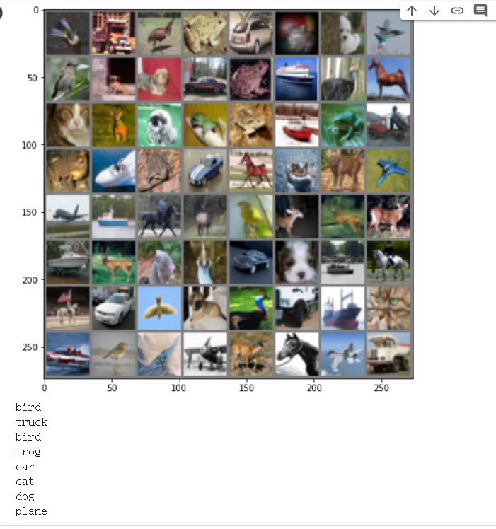
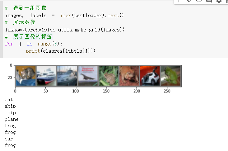
def imshow(img):
    plt.figure(figsize=(8,8))
    img = img / 2 + 0.5     # 转换到 [0,1] 之间
    npimg = img.numpy()
    plt.imshow(np.transpose(npimg, (1, 2, 0)))
    plt.show()

# 得到一组图像
images, labels = iter(trainloader).next()
# 展示图像
imshow(torchvision.utils.make_grid(images))
# 展示第一行图像的标签
for j in range(8):
    print(classes[labels[j]])

class Net(nn.Module):
    def __init__(self):
        super(Net, self).__init__()
        self.conv1 = nn.Conv2d(3, 6, 5)
        self.pool = nn.MaxPool2d(2, 2)
        self.conv2 = nn.Conv2d(6, 16, 5)
        self.fc1 = nn.Linear(16 * 5 * 5, 120)
        self.fc2 = nn.Linear(120, 84)
        self.fc3 = nn.Linear(84, 10)

    def forward(self, x):
        x = self.pool(F.relu(self.conv1(x)))
        x = self.pool(F.relu(self.conv2(x)))
        x = x.view(-1, 16 * 5 * 5)
        x = F.relu(self.fc1(x))
        x = F.relu(self.fc2(x))
        x = self.fc3(x)
        return x

# 网络放到GPU上
net = Net().to(device)
criterion = nn.CrossEntropyLoss()
optimizer = optim.Adam(net.parameters(), lr=0.001)

for epoch in range(10):  # 重复多轮训练
    for i, (inputs, labels) in enumerate(trainloader):
        inputs = inputs.to(device)
        labels = labels.to(device)
        # 优化器梯度归零
        optimizer.zero_grad()
        # 正向传播 +　反向传播 + 优化 
        outputs = net(inputs)
        loss = criterion(outputs, labels)
        loss.backward()
        optimizer.step()
        # 输出统计信息
        if i % 100 == 0:   
            print('Epoch: %d Minibatch: %5d loss: %.3f' %(epoch + 1, i + 1, loss.item()))

print('Finished Training')

 

 

 

 

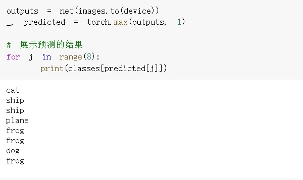
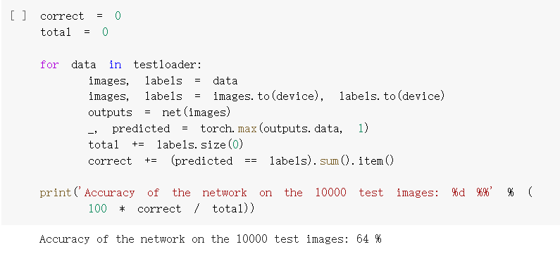
准确率64%

三、使用 VGG16 对 CIFAR10 分类

1.

2.

cfg = [64, 'M', 128, 'M', 256, 256, 'M', 512, 512, 'M', 512, 512, 'M']
class VGG(nn.Module):
    def __init__(self):
        super(VGG, self).__init__()
        #self.cfg = [64, 'M', 128, 'M', 256, 256, 'M', 512, 512, 'M', 512, 512, 'M']
        self.features = self._make_layers(cfg)
        #self.classifier = nn.Linear(2048, 10)
        self.classifier = nn.Linear(512, 10)

    def forward(self, x):
        out = self.features(x)
        out = out.view(out.size(0), -1)
        out = self.classifier(out)
        return out

    def _make_layers(self, cfg):
        layers = []
        in_channels = 3
        for x in cfg:
            if x == 'M':
                layers += [nn.MaxPool2d(kernel_size=2, stride=2)]
            else:
                layers += [nn.Conv2d(in_channels, x, kernel_size=3, padding=1),
                           nn.BatchNorm2d(x),
                           nn.ReLU(inplace=True)]
                in_channels = x
        layers += [nn.AvgPool2d(kernel_size=1, stride=1)]
        return nn.Sequential(*layers)

net = VGG().to(device)
criterion = nn.CrossEntropyLoss()
optimizer = optim.Adam(net.parameters(), lr=0.001)

3.

for epoch in range(10):  # 重复多轮训练
    for i, (inputs, labels) in enumerate(trainloader):
        inputs = inputs.to(device)
        labels = labels.to(device)
        # 优化器梯度归零
        optimizer.zero_grad()
        # 正向传播 +　反向传播 + 优化 
        outputs = net(inputs)
        loss = criterion(outputs, labels)
        loss.backward()
        optimizer.step()
        # 输出统计信息
        if i % 100 == 0:   
            print('Epoch: %d Minibatch: %5d loss: %.3f' %(epoch + 1, i + 1, loss.item()))

print('Finished Training')

 

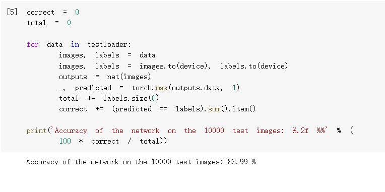
准确率为83.99%，相较之前有所提升。