UFLDL学习笔记 ---- 主成分分析与白化

主成分分析（PCA）是用来提升无监督特征学习速度的数据降维算法。看过下文大致可以知道，PCA本质是对角化协方差矩阵，目的是让维度之间的相关性最小（降噪），保留下来的维度能量最大（去冗余），PCA在图像数据的降维上很实用，因为图像数据相邻元素的相关性是很高的。

为了方便解释，我们以二维数据降一维为例（实际应用可能需要把数据从256降到50）：

 

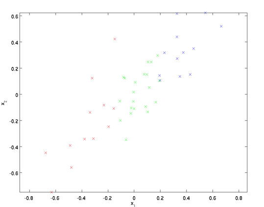
需要注意的是，两个特征值经过了预处理，其均值为零，方差相等，下文会解释其原因，不过在图像处理上，方差的预处理过程就没必要了。

 

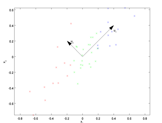
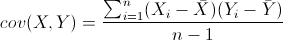
从上图可以看出，数据主要向两个方向变化，即u1 u2，PCA算法需要用到协方差的运算，（方差是同一类或者说同一维数据的离散性，而协方差则是不同维度数据的相关性，协方差为0说明二者独立不相关，为负就是负相关，为正就是正相关）。协方差的公式为：

 

PCA用到的公式为：

 

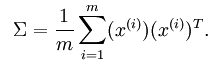
这也就是为什么需要将数据均值预处理为零的原因，注意等号左边的不是求和符号，读作sigma，是协方差矩阵的标准符号。

可以证明数据变化的主方向u1就是协方差矩阵的主特征向量，而u2就是次特征向量（原理有兴趣的同学请看这里）。求协方差矩阵以及其特征向量的过程在各种线代库都有提供，不需要手动实现，Matlab中可以使用[U,S,D]=svd(sigma)（简单解释下sigma做参数的原因，PCA关心的是矩阵x的变化方向，其转化结果要具有最大方差，也就可以通过求协方差的变化方向来确定），svd函数是用来求矩阵奇异值分解的，这里用来求特征值大致是因为实数域对称矩阵的特征值的绝对值和奇异值相等。

这里我们是要降为一维，所以就使用u1就好，也就是说，降到几维就使用前几个特征向量。

 

上图对应了n个特征向量，特征值的标准符号是  ，在主成分个数选择中会用到，其公式为： 。

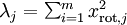旋转

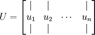
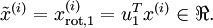
对于本例来说，旋转数据就是将数据重新放在以 和 为轴的坐标系里，表达式为：

 

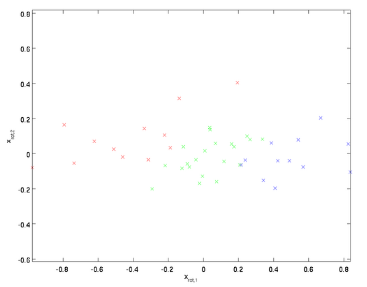
旋转后的坐标如下图：

 

矩阵U有正交性，满足  ，所以要将旋转后的数据还原，只需左乘U即可：   , 验证：  。

降维

有了上面的铺垫，降维操作就容易理解了，本例的公式为：

 

推广到一般情况就是取矩阵U的前K个特征向量就可以降到K维了，可以这样看，PCA算法的特征向量越靠后对数据的影响越小，降维就是取其中靠前的重要数据，从而达到下图的效果：

 

降维后的坐标系：

 

主成分个数选择

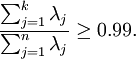
主成分个数K的选择显然是最重要的了，我们的做法是在给定一个百分比，可以是99%或者95%等，自己定，然后计算前K个特征值的和占所有特征值的百分比，如果超过了给定的百分比则可以选定这K个值作为主成分个数。

 

对图像数据使用PCA

正如之前提及的，使用PCA算法通常需要对数据做预处理使每个特征的均值为零、方差相近。但是对于大部分图像类型，我们不需要预处理过程，因为理论上图像任意部分的统计性质都和其它部分相同，图像的这种特性被称作平稳性。

总的来说，即使不对图像做方差归一化操作，也可以满足不同特征的方差值彼此相近（对于音频如声谱，文本如词袋向量，通常也不进行方差归一化）。实际上，PCA对于输入数据具有缩放不变性，无论输入数据值被 如何放大缩小，返回的特征向量都一样。

至于均值规整为0，则要依赖于不同的应用处理，例如物体检测，我们通常并不关心亮度这个特征，因为亮度并不影响物体检测的结果，所以这里的规整操作就是把将样本每个亮度值减去样本的平均亮度值，如下图公式：

 

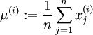
, for all 

请注意：1）对每个输入图像块都要单独执行上面两个步骤，2）这里的   是指图像块  的平均亮度值。尤其需要注意的是，这和为每个像素  单独估算均值是两个完全不同的概念。

如果处理的图像并非自然图像（比如，手写文字，或者白背景正中摆放单独物体），其他规整化操作就值得考虑了，而哪种做法最合适也取决于具体应用场合。但对自然图像而言，对每幅图像进行上述的零均值规整化，是默认而合理的处理。

白化

白化是数据预处理过程，用来降低输入的冗余性，起作用可以概括为：

• 减少特征之间的相关性
• 特征方差相近

依然以二维的例子来解释，实际上前文旋转操作  的操作已经消除了输入特征的相关性，再看一下之前的坐标系图：

 

其协方差矩阵为：

 

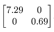
（注意，本文中所有的协方差计算，输入特征的均值默认为零，当然，即使均值不为零，下面介绍的理论依然通用）

观察上面的矩阵，对角元素的值为lambda1和lambda2以及次对角元素为0绝非偶然，由次对角0知道 和  不相关，满足降低不同维度的相关性这一条。

为了使输入特征具有单位方差，我们可以做如下操作以实现白化，这里lambda实际上就等于旋转后的矩阵的方差值：

 

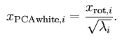
白化后的坐标图：

 

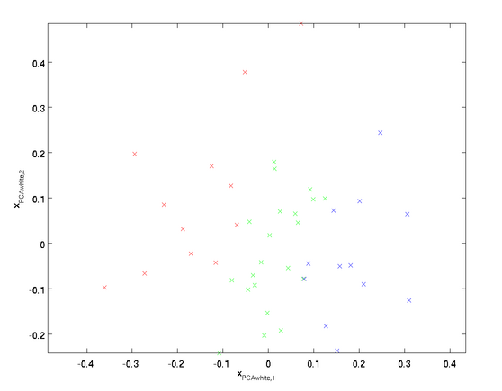
这个操作之后，协方差矩阵就变为了单位矩阵I，此时的  就称为PCA白化后的版本。

注意，这里并没有对数据进行降维，只是做了旋转操作，如果想结合降维，只需保留xPCAWhite的前K项即可。

ZCA白化

首先应该知道，如果R是任意正交矩阵，那么 仍然具有单位协方差。在ZCA白化中，令R=U（由上文知，U本身就是正交矩阵），其定义为：

 

也就是在原来PCA结果上（不降维）左乘一个特征向量矩阵，ZCA白化的坐标系：

 

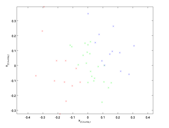
可以证明，对所有可能的R，这种旋转使得  尽可能地接近原始数据x。

当使用ZCA白化时，我们通常保留数据的全部n个维度，不尝试去降低他的维度。

 

正则化

实践中需要实现PCA白化或ZCA白化时，有时一些特征值   在数值上接近于0，这样在缩放步骤时我们除以   将导致除以一个接近0的值；这可能使数据上溢 (赋为大数值)或造成数值不稳定。因而在实践中，我们使用少量的正则化实现这个缩放过程，即在取平方根和倒数之前给特征值加上一个很小的常数  ：

 

当 x  在区间   上时, 一般取值为  。

对图像来说, 这里加上   ，对输入图像也有一些平滑(或低通滤波)的作用。这样处理还能消除在图像的像素信息获取过程中产生的噪声，改善学习到的特征(细节超出了本文的范围)。

ZCA 白化是一种数据预处理方法，它将数据从   映射到   。 事实证明这也是一种生物眼睛(视网膜)处理图像的粗糙模型。具体而言，当你的眼睛感知图像时，由于一幅图像中相邻的部分在亮度上十分相关，大多数临近的“像素”在眼中被感知为相近的值。因此，如果人眼需要分别传输每个像素值（通过视觉神经）到大脑中，会非常不划算。取而代之的是，视网膜进行一个与ZCA中相似的去相关操作 (这是由视网膜上的ON-型和OFF-型光感受器细胞将光信号转变为神经信号完成的)。由此得到对输入图像的更低冗余的表示，并将它传输到大脑。

 

练习

pca_2d

close all

%%================================================================
%% Step 0: Load data
%  We have provided the code to load data from pcaData.txt into x.
%  x is a 2 * 45 matrix, where the kth column x(:,k) corresponds to
%  the kth data point.Here we provide the code to load natural image data into x.
%  You do not need to change the code below.

x = load('pcaData.txt','-ascii');
figure(1);
scatter(x(1, :), x(2, :));
title('Raw data');


%%================================================================
%% Step 1a: Implement PCA to obtain U 
%  Implement PCA to obtain the rotation matrix U, which is the eigenbasis
%  sigma. 

% -------------------- YOUR CODE HERE -------------------- 
u = zeros(size(x, 1)); % You need to compute this
conv = (1/size(x,1))*(x'*x);
[u,s,d] = svd(conv);

% -------------------------------------------------------- 
hold on
plot([0 u(1,1)], [0 u(2,1)]);
plot([0 u(1,2)], [0 u(2,2)]);
scatter(x(1, :), x(2, :));
hold off

%%================================================================
%% Step 1b: Compute xRot, the projection on to the eigenbasis
%  Now, compute xRot by projecting the data on to the basis defined
%  by U. Visualize the points by performing a scatter plot.

% -------------------- YOUR CODE HERE -------------------- 
xRot = zeros(size(x)); % You need to compute this
xRot = u'*x;

% -------------------------------------------------------- 

% Visualise the covariance matrix. You should see a line across the
% diagonal against a blue background.
figure(2);
scatter(xRot(1, :), xRot(2, :));
title('xRot');

%%================================================================
%% Step 2: Reduce the number of dimensions from 2 to 1. 
%  Compute xRot again (this time projecting to 1 dimension).
%  Then, compute xHat by projecting the xRot back onto the original axes 
%  to see the effect of dimension reduction

% -------------------- YOUR CODE HERE -------------------- 
k = 1; % Use k = 1 and project the data onto the first eigenbasis
xHat = zeros(size(x)); % You need to compute this
xRot = u(:,1)'*x;
xHat = u*[xRot;zeros(1,size(x,2))];

% -------------------------------------------------------- 
figure(3);
scatter(xHat(1, :), xHat(2, :));
title('xHat');


%%================================================================
%% Step 3: PCA Whitening
%  Complute xPCAWhite and plot the results.

epsilon = 1e-5;
% -------------------- YOUR CODE HERE -------------------- 
xPCAWhite = zeros(size(x)); % You need to compute this 
xRot = u'*x;
xPCAWhite = diag(1./sqrt(diag(s) + epsilon)) * xRot;

% -------------------------------------------------------- 
figure(4);
scatter(xPCAWhite(1, :), xPCAWhite(2, :));
title('xPCAWhite');

%%================================================================
%% Step 3: ZCA Whitening
%  Complute xZCAWhite and plot the results.

% -------------------- YOUR CODE HERE -------------------- 
xZCAWhite = zeros(size(x)); % You need to compute this
xZCAWhite = u*xPCAWhite;

% -------------------------------------------------------- 
figure(5);
scatter(xZCAWhite(1, :), xZCAWhite(2, :));
title('xZCAWhite');

%% Congratulations! When you have reached this point, you are done!
%  You can now move onto the next PCA exercise. :)

PCA and Whitening

%%================================================================
%% Step 0a: Load data
%  Here we provide the code to load natural image data into x.
%  x will be a 144 * 10000 matrix, where the kth column x(:, k) corresponds to
%  the raw image data from the kth 12x12 image patch sampled.
%  You do not need to change the code below.

x = sampleIMAGESRAW();
figure('name','Raw images');
randsel = randi(size(x,2),200,1); % A random selection of samples for visualization
display_network(x(:,randsel));

%%================================================================
%% Step 0b: Zero-mean the data (by row)
%  You can make use of the mean and repmat/bsxfun functions.

% -------------------- YOUR CODE HERE -------------------- 

x = bsxfun(@minus,x,mean(x,1)); % use bsxfun
%x = x-repmat(mean(x,1),size(x,1),1); % use repmat

%%================================================================
%% Step 1a: Implement PCA to obtain xRot
%  Implement PCA to obtain xRot, the matrix in which the data is expressed
%  with respect to the eigenbasis of sigma, which is the matrix U.


% -------------------- YOUR CODE HERE -------------------- 
xRot = zeros(size(x)); % You need to compute this
[U,S,D] = svd(x*x'*(1/size(x,2)));
xRot = U'*x;

%%================================================================
%% Step 1b: Check your implementation of PCA
%  The covariance matrix for the data expressed with respect to the basis U
%  should be a diagonal matrix with non-zero entries only along the main
%  diagonal. We will verify this here.
%  Write code to compute the covariance matrix, covar. 
%  When visualised as an image, you should see a straight line across the
%  diagonal (non-zero entries) against a blue background (zero entries).

% -------------------- YOUR CODE HERE -------------------- 
covar = zeros(size(x, 1)); % You need to compute this
covar = xRot*xRot'*(1/size(xRot,2)); % equal to S

% Visualise the covariance matrix. You should see a line across the
% diagonal against a blue background.
figure('name','Visualisation of covariance matrix');
imagesc(covar);

%%================================================================
%% Step 2: Find k, the number of components to retain
%  Write code to determine k, the number of components to retain in order
%  to retain at least 99% of the variance.

% -------------------- YOUR CODE HERE -------------------- 
k = 1; % Set k accordingly
diag_vec = diag(S);
k=length(diag_vec((cumsum(diag_vec)./sum(diag_vec))<0.99));

%%================================================================
%% Step 3: Implement PCA with dimension reduction
%  Now that you have found k, you can reduce the dimension of the data by
%  discarding the remaining dimensions. In this way, you can represent the
%  data in k dimensions instead of the original 144, which will save you
%  computational time when running learning algorithms on the reduced
%  representation.
% 
%  Following the dimension reduction, invert the PCA transformation to produce 
%  the matrix xHat, the dimension-reduced data with respect to the original basis.
%  Visualise the data and compare it to the raw data. You will observe that
%  there is little loss due to throwing away the principal components that
%  correspond to dimensions with low variation.

% -------------------- YOUR CODE HERE -------------------- 
xHat = zeros(size(x));  % You need to compute this
xReduction = U(:,1:k)' * x;
xHat(1:k,:)=xReduction;
xHat=U*xHat;

% Visualise the data, and compare it to the raw data
% You should observe that the raw and processed data are of comparable quality.
% For comparison, you may wish to generate a PCA reduced image which
% retains only 90% of the variance.

figure('name',['PCA processed images ',sprintf('(%d / %d dimensions)', k, size(x, 1)),'']);
display_network(xHat(:,randsel));
figure('name','Raw images');
display_network(x(:,randsel));

%%================================================================
%% Step 4a: Implement PCA with whitening and regularisation
%  Implement PCA with whitening and regularisation to produce the matrix
%  xPCAWhite. 

epsilon = 0.1;
xPCAWhite = zeros(size(x));
% -------------------- YOUR CODE HERE -------------------- 
xPCAWhite = diag(1./sqrt(diag(S) + epsilon)) * U' * x;

%%================================================================
%% Step 4b: Check your implementation of PCA whitening 
%  Check your implementation of PCA whitening with and without regularisation. 
%  PCA whitening without regularisation results a covariance matrix 
%  that is equal to the identity matrix. PCA whitening with regularisation
%  results in a covariance matrix with diagonal entries starting close to 
%  1 and gradually becoming smaller. We will verify these properties here.
%  Write code to compute the covariance matrix, covar. 
%
%  Without regularisation (set epsilon to 0 or close to 0), 
%  when visualised as an image, you should see a red line across the
%  diagonal (one entries) against a blue background (zero entries).
%  With regularisation, you should see a red line that slowly turns
%  blue across the diagonal, corresponding to the one entries slowly
%  becoming smaller.

% -------------------- YOUR CODE HERE -------------------- 
covar = zeros(size(xPCAWhite, 1));
covar = xPCAWhite*xPCAWhite'*(1./size(xPCAWhite,2));
% Visualise the covariance matrix. You should see a red line across the
% diagonal against a blue background.
figure('name','Visualisation of covariance matrix');
imagesc(covar);

%%================================================================
%% Step 5: Implement ZCA whitening
%  Now implement ZCA whitening to produce the matrix xZCAWhite. 
%  Visualise the data and compare it to the raw data. You should observe
%  that whitening results in, among other things, enhanced edges.

xZCAWhite = zeros(size(x));

% -------------------- YOUR CODE HERE -------------------- 
xZCAWhite=U * diag(1./sqrt(diag(S) + epsilon)) * U' * x;
% Visualise the data, and compare it to the raw data.
% You should observe that the whitened images have enhanced edges.
figure('name','ZCA whitened images');
display_network(xZCAWhite(:,randsel));
figure('name','Raw images');
display_network(x(:,randsel));