
Python爬虫可视化分析之2021年11月的全国火力发电量情况
Python爬虫可视化分析之20210年11月的全国火力发电量
(一)选题的背景
我所选择是2021年全国部分月数的火力发电量情况,随着疫情有所缓解,全国工业开始慢慢复苏,想更加了解一些企业的用电量和发电量是否成比例关系或者正、负相关。我所要达到的数据分析的预期目标是让人们初步了解我国各省市的基本火力发电情况,随着全球气温变暖,让人们时时刻刻有所警惕,能更加直观的清晰的展现在人们面前。
(二)主题是网络爬虫设计方案
(1)主题是网络爬虫名称:2021年全国部分月数的火力发电量
(2)主题是网络爬虫爬取的内容与数据特征分析:
爬取该网站的当月产量(亿千瓦小时)、累计产量(亿千瓦小时)、当月同比增长(%)、累计增长(%) 等做数据可视化分析
(3)主题是网络爬虫设计方案的概述
爬取所在网站的产量以及增长率 并 找到该标签下的内容整合到列表中,在使用pandas中的数据表格分析和综合排名,进行数据的可视化分析等。具体的思路和爬取过程分析如下代码和截图图片展示。
(三)主题页面的结构特征分析
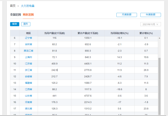
(1)数据源来自 中商产业研究院的数据库
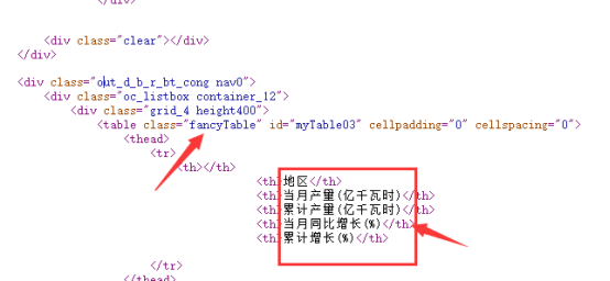
(2)主题页面的结构与特征分析和html 的页面解析
红色方框中 是 我所提取的列名
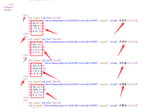
找到<tbody>标签下的<tr>标签 用get_text() 或者 text 获得其标签中的内容,并用遍历的方式逐一打印出来

每个省市所对应的当月产量、累计产量、当月的同比增长以及累计增长 都在该标签下,用正则表达式或者BeautifulSoup 来获取所需的数据
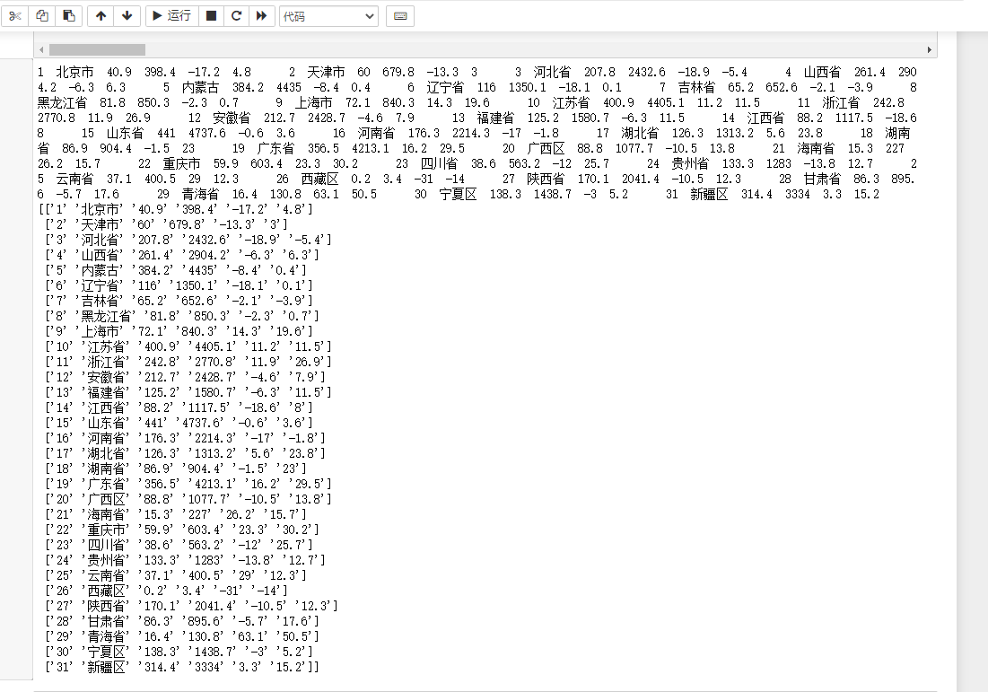
所对应爬取的数据
(四)数据清洗
主要步骤:
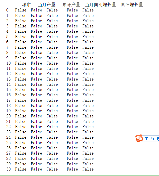
1、查看数据是否为空值
2、查看数据是否缺失
 1 #数据的清理和处理
 2 from pandas import DataFrame,Series
 3 import pandas as pd
 4 import numpy as np
 5 df_first = DataFrame(data)
 6
 7 # 检查数据缺值
 8 print(df_first.isnull())
 9
10 #检查数据 是否有出现 空值
11 df_first.notnull()

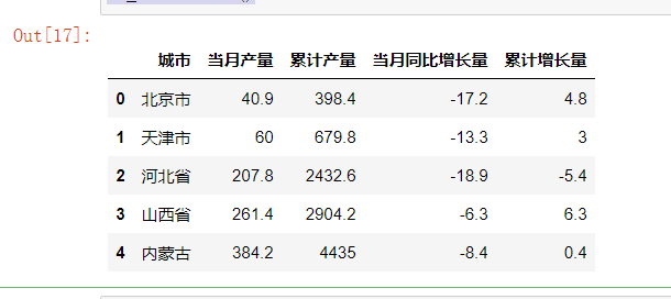
1 #前五个的数据
2 df_first.head()
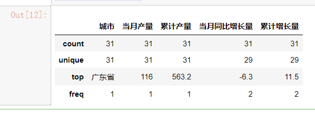
1 # top 榜和各个数据的对比 2 df_first.describe()
1 #通过sum可以获得每一列的缺失值数量,在通过sum可以获得整个DataFrame的缺失值数量
2 df_first.isnull().sum()

1 #通过info的方法可以获得整个DataFrame的数据缺失情况 2 df_first.info()

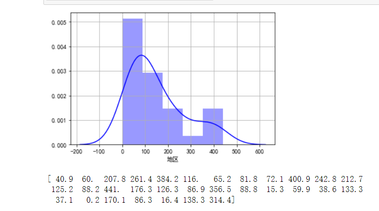
 1 import seaborn as sns
 2 import matplotlib.pyplot as plt
 3 import warnings
 4 # 忽略运行 警告处理
 5 warnings.filterwarnings("ignore")
 6
 7 #导入excel表中的数据
 8 res_electric = pd.read_excel('D:\\code\\res.xlsx')
 9 plt.figure
10
11 # 频率分布直方图
12 sns.distplot(res_electric['当月产量'].values,hist = True, rug = False, fit = None,
13              axlabel = '地区',
14              label = '火力发电产量',
15              hist_kws = {'color':'b'},
16              kde_kws = {'color':'b' } )
17 res_electric['当月产量'].values
18 plt.ylabel('')
19 plt.grid(linestyle = '-')
20 plt.show()
21 print(res_electric['当月产量'].values)
 1 # 柱状图 :全国各个地区的当月产量
 2 plt.rcParams['font.sans-serif'] = ['SimHei'] #
 3 plt.rcParams['axes.unicode_minus'] = False
 4 x = citys
 5 y = yields
 6 plt.bar(x, y, width=0.7)
 7 plt.xticks(x, x, rotation=70)
 8 plt.bar(x, y,color = 'b')
 9 plt.title('全国各个地区的当月产量')
10 plt.show()

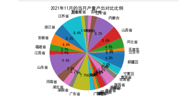
 1 import matplotlib.pyplot as plt
 2 Type = citys
 3 Data = yields
 4 #cols = ['r','g','y','coral']
 5 #绘制饼图
 6 plt.pie(Data ,labels=Type, autopct='%1.1f%%')
 7 #设置显示图像为圆形
 8 plt.axis('equal')
 9 plt.title('2021年11月的当月产量产出对比比例')
10 plt.show()
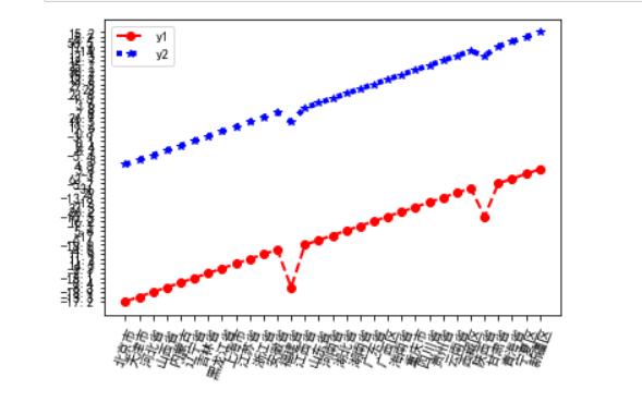
 1 # 创建figure对象  , 并展示出当月同比增长量、累计增长量
 2 plt.figure()
 3 # 绘制普通图像
 4 x = citys
 5 y1 = increases
 6 y2 = allIncreases
 7 plt.xticks(rotation=70)
 8 # 绘制y1,线条说明为'y1',线条宽度为2,颜色为红色,线型为虚线,数据标记为圆圈
 9 plt.plot(x, y1, label='y1',linewidth = 2, linestyle='--', marker='o', color='r')
10 # 绘制y2,线条说明为'y2',线条宽度为4,颜色为蓝色,线型为点线,数据标记为'*'
11 plt.plot(x, y2,'b:*',label='y2',linewidth = 4)
12 # 显示图例
13 plt.legend()
14 # 显示图像
15 plt.show()
 1 #  圆环图 类似于 扇形
 2 # 创建数据
 3 size_of_groups = allYields
 4 # 生成饼图
 5 plt.pie(size_of_groups)
 6 # 在中心添加一个圆, 生成环形图展现数据的分布比例
 7 my_circle = plt.Circle((0, 0), 0.7, color='white')
 8 p = plt.gcf()
 9 p.gca().add_artist(my_circle)
10 plt.show()

1 # 设置圆点大小
2 size =  50
3 # 绘制散点图
4 plt.scatter(citys,increases , size, color="r", alpha=0.5, marker='o')
5 plt.xticks(x, x, rotation=70)
6 plt.xlabel("地 区")
7 plt.ylabel("累计增长量")
8 plt.title("2021年11月全国各个地区的火力发电情况")
9 plt.show()

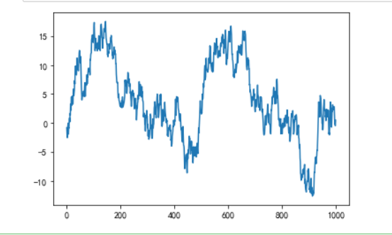
1  # 折线图
2 data = pd.Series(np.random.randn(1000),index=np.arange(1000))
3 data = data.cumsum()
4 data.plot()
5 plt.show()
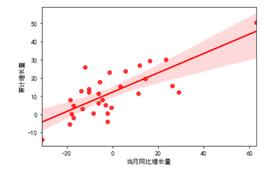
1  # 拟合线性曲线
2 sns.regplot(res_electric['当月同比增长量'],res_electric['累计增长量'],color = 'r')
3 plt.show()
 1 #计算回归方程系数、截距、线性回归预测模型表达式
 2 from sklearn import datasets
 3 from sklearn.linear_model import LinearRegression
 4 from sklearn.datasets import load_boston
 5
 6 predict_model = LinearRegression()
 7 X = res_electric['当月产量'].values
 8 X = X.reshape(-1,1)
 9 predict_model.fit(X , res_electric['累计产量'])
10 np.set_printoptions(precision = 3, suppress = True)
11 a = predict_model.coef_
12 b = predict_model.intercept_
13 print("回归方程系数{}".format(predict_model.coef_))
14 print("回归方程截距{0:2f}".format(predict_model.intercept_))
15 print("线性回归预测模型表达式为{}*x+{}".format(predict_model.coef_,predict_model.intercept_))

  1 import re
  2 import requests
  3 from bs4 import BeautifulSoup
  4 import time
  5 from requests.exceptions import RequestException
  6 import numpy as np
  7 import pandas as pd
  8
  9
 10 def getPage(url):
 11     # 爬取指定的url地址对应的页面信息
 12     # 进行异常处理,防止网页没有反应,等待时长过久
 13     try:
 14         # 封装请求头信息
 15         headers = {
 16             'User-Agent': 'Mozilla/5.0 (Windows NT 10.0; Win64; x64) AppleWebKit/537.36(KHTML, like Gecko) Chrome/96.0.4664.110 Safari/537.36'
 17         }
 18         res = requests.get(url, headers=headers)
 19         # 判断网页请求是否成功
 20         if res.status_code == 200:
 21             res.encoding = 'utf-8'
 22             return res.text
 23         else:
 24             return None
 25     except RequestException:
 26         return None
 27
 28
 29 def parsePage(html):
 30     # 解析爬取网页内容,并返回字段结果
 31     # 解析出各个数据的列名
 32     soup = BeautifulSoup(html, "lxml")
 33     hang = soup.tr.text
 34     hang_list = []
 35     hang_list.append(hang.replace("\n", " "))
 36     # 解析出各个地区对应的数据
 37     Datas = soup.tbody.text.replace("\n", "  ")
 38
 39     #函数使用
 40     writeFile(Datas)
 41
 42
 43 #函数调用 将Datas数据 写入excel 表格中
 44 def writeFile(Datas):
 45
 46     lines = Datas.split("      ")
 47     Datas = []
 48     for line in lines:
 49         dataLine = line.split("  ")
 50         dataLine = np.array(dataLine,dtype=object)
 51         Datas.append(dataLine)
 52     Datas[0] = Datas[0][2:]
 53     Datas[-1] = Datas[-1][:-2]
 54     Datas = np.array(Datas,dtype=object)
 55
 56     #各个列名所需的数据如下
 57     citys = Datas[:,1]
 58     yields = Datas[:,2]
 59     allYields = Datas[:,3]
 60     increases = Datas[:,4]
 61     allIncreases = Datas[:,5]
 62
 63     data = {"城市":citys,"当月产量":yields,"累计产量":allYields,"当月同比增长量":increases,"累计增长量":allIncreases}
 64     df = pd.DataFrame(data)
 65     df.to_excel("res.xlsx")
 66
 67
 68 # 爬虫的主函数(调度)
 69 def main():
 70     url = 'https://s.askci.com/data/shengenergy/a03010h/'
 71     html = getPage(url)
 72     if html:
 73         parsePage(html)
 74     else:
 75         return None
 76
 77 if __name__ == '__main__':
 78     main()
 79
 80 import numpy as np
 81 import pandas as pd
 82
 83 datas = """1  北京市  40.9  398.4  -17.2  4.8      2  天津市  60  679.8  -13.3  3      3  河北省  207.8  2432.6  -18.9  -5.4      4  山西省  261.4  2904.2  -6.3  6.3      5  内蒙古  384.2  4435  -8.4  0.4      6  辽宁省  116  1350.1  -18.1  0.1      7  吉林省  65.2  652.6  -2.1  -3.9      8  黑龙江省  81.8  850.3  -2.3  0.7      9  上海市  72.1  840.3  14.3  19.6      10  江苏省  400.9  4405.1  11.2  11.5      11  浙江省  242.8  2770.8  11.9  26.9      12  安徽省  212.7  2428.7  -4.6  7.9      13  福建省  125.2  1580.7  -6.3  11.5      14  江西省  88.2  1117.5  -18.6  8      15  山东省  441  4737.6  -0.6  3.6      16  河南省  176.3  2214.3  -17  -1.8      17  湖北省  126.3  1313.2  5.6  23.8      18  湖南省  86.9  904.4  -1.5  23      19  广东省  356.5  4213.1  16.2  29.5      20  广西区  88.8  1077.7  -10.5  13.8      21  海南省  15.3  227  26.2  15.7      22  重庆市  59.9  603.4  23.3  30.2      23  四川省  38.6  563.2  -12  25.7      24  贵州省  133.3  1283  -13.8  12.7      25  云南省  37.1  400.5  29  12.3      26  西藏区  0.2  3.4  -31  -14      27  陕西省  170.1  2041.4  -10.5  12.3      28  甘肃省  86.3  895.6  -5.7  17.6      29  青海省  16.4  130.8  63.1  50.5      30  宁夏区  138.3  1438.7  -3  5.2      31  新疆区  314.4  3334  3.3  15.2"""
 84 lines = datas.split("      ")
 85 datas = []
 86 for line in lines:
 87     dataLine = line.split("  ")
 88     dataLine = np.array(dataLine)
 89     datas.append(dataLine)
 90 datas = np.array(datas)
 91 #%%
 92
 93 datas
 94 citys = datas[:,1]
 95 yields = datas[:,2]
 96 allYields = datas[:,3]
 97 increases = datas[:,4]
 98 allIncreases = datas[:,5]
 99 data = {"城市":citys,"当月产量":yields,"累计产量":allYields,"当月同比增长量":increases,"累计增长量":allIncreases}
100 df = pd.DataFrame(data)
101 df.to_excel("res.xlsx")
102
103 #数据的清理和处理
104 from pandas import DataFrame,Series
105 import pandas as pd
106 import numpy as np
107 df_first = DataFrame(data)
108
109 # 检查数据缺值
110 print(df_first.isnull())
111
112 #检查数据 是否有出现 空值
113 df_first.notnull()
114
115 #前五个的数据
116 df_first.head()
117
118 # top 榜和各个数据的对比
119 df_first.describe()
120
121 #通过sum可以获得每一列的缺失值数量,在通过sum可以获得整个DataFrame的缺失值数量
122 df_first.isnull().sum()
123
124 #通过info的方法可以获得整个DataFrame的数据缺失情况
125 df_first.info()
126
127 import seaborn as sns
128 import matplotlib.pyplot as plt
129 import warnings
130 # 忽略运行 警告处理
131 warnings.filterwarnings("ignore")
132
133 #导入excel表中的数据
134 res_electric = pd.read_excel('D:\\code\\res.xlsx')
135 plt.figure
136
137 # 频率分布直方图
138 sns.distplot(res_electric['当月产量'].values,hist = True, rug = False, fit = None,
139              axlabel = '地区',
140              label = '火力发电产量',
141              hist_kws = {'color':'b'},
142              kde_kws = {'color':'b' } )
143 res_electric['当月产量'].values
144 plt.ylabel('')
145 plt.grid(linestyle = '-')
146 plt.show()
147 print(res_electric['当月产量'].values)
148
149 # 柱状图 :全国各个地区的当月产量
150 plt.rcParams['font.sans-serif'] = ['SimHei'] #
151 plt.rcParams['axes.unicode_minus'] = False
152 x = citys
153 y = yields
154 plt.bar(x, y, width=0.7)
155 plt.xticks(x, x, rotation=70)
156 plt.bar(x, y,color = 'b')
157 plt.title('全国各个地区的当月产量')
158 plt.show()
159
160 import matplotlib.pyplot as plt
161 Type = citys
162 Data = yields
163 #cols = ['r','g','y','coral']
164 #绘制饼图
165 plt.pie(Data ,labels=Type, autopct='%1.1f%%')
166 #设置显示图像为圆形
167 plt.axis('equal')
168 plt.title('2021年11月的当月产量产出对比比例')
169 plt.show()
170
171 # 创建figure对象  , 并展示出当月同比增长量、累计增长量
172 plt.figure()
173 # 绘制普通图像
174 x = citys
175 y1 = increases
176 y2 = allIncreases
177 plt.xticks(rotation=70)
178 # 绘制y1,线条说明为'y1',线条宽度为2,颜色为红色,线型为虚线,数据标记为圆圈
179 plt.plot(x, y1, label='y1',linewidth = 2, linestyle='--', marker='o', color='r')
180 # 绘制y2,线条说明为'y2',线条宽度为4,颜色为蓝色,线型为点线,数据标记为'*'
181 plt.plot(x, y2,'b:*',label='y2',linewidth = 4)
182 # 显示图例
183 plt.legend()
184 # 显示图像
185 plt.show()
186
187 #  圆环图 类似于 扇形
188 # 创建数据
189 size_of_groups = allYields
190 # 生成饼图
191 plt.pie(size_of_groups)
192 # 在中心添加一个圆, 生成环形图
193 my_circle = plt.Circle((0, 0), 0.7, color='white')
194 p = plt.gcf()
195 p.gca().add_artist(my_circle)
196 plt.show()
197
198 # 设置圆点大小
199 size =  50
200 # 绘制散点图
201 plt.scatter(citys,increases , size, color="r", alpha=0.5, marker='o')
202 plt.xticks(x, x, rotation=70)
203 plt.xlabel("地 区")
204 plt.ylabel("累计增长量")
205 plt.title("2021年11月全国各个地区的火力发电情况")
206 plt.show()
207
208  # 折线图
209 data = pd.Series(np.random.randn(1000),index=np.arange(1000))
210 data = data.cumsum()
211 data.plot()
212 plt.show()
213
214  # 拟合线性曲线
215 sns.regplot(res_electric['当月同比增长量'],res_electric['累计增长量'],color = 'r')
216 plt.show()
217
218 #计算回归方程系数、截距、线性回归预测模型表达式
219 from sklearn import datasets
220 from sklearn.linear_model import LinearRegression
221 from sklearn.datasets import load_boston
222
223 predict_model = LinearRegression()
224 X = res_electric['当月产量'].values
225 X = X.reshape(-1,1)
226 predict_model.fit(X , res_electric['累计产量'])
227 np.set_printoptions(precision = 3, suppress = True)
228 a = predict_model.coef_
229 b = predict_model.intercept_
230 print("回归方程系数{}".format(predict_model.coef_))
231 print("回归方程截距{0:2f}".format(predict_model.intercept_))
232 print("线性回归预测模型表达式为{}*x+{}".format(predict_model.coef_,predict_model.intercept_))

