

Andrew Ng机器学习 四:Neural Networks Learning
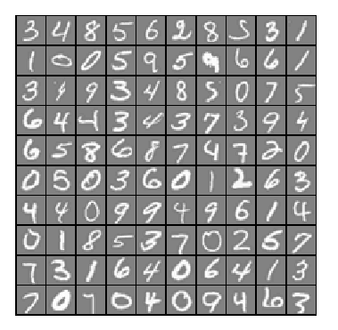
背景:跟上一讲一样,识别手写数字,给一组数据集ex4data1.mat,,每个样例都为灰度化为20*20像素,也就是每个样例的维度为400,加载这组数据后,我们会有5000*400的矩阵X(5000个样例),5000*1的矩阵y(表示每个样例所代表的数据)。现在让你拟合出一个模型,使得这个模型能很好的预测其它手写的数字。
(注意:我们用10代表0(矩阵y也是这样),因为Octave的矩阵没有0行)
一:神经网络( Neural Networks)
神经网络脚本ex4.m:


%% Machine Learning Online Class - Exercise 4 Neural Network Learning

%  Instructions
%  ------------
%
%  This file contains code that helps you get started on the
%  linear exercise. You will need to complete the following functions
%  in this exericse:
%
%     sigmoidGradient.m
%     randInitializeWeights.m
%     nnCostFunction.m
%
%  For this exercise, you will not need to change any code in this file,
%  or any other files other than those mentioned above.
%

%% Initialization
clear ; close all; clc

%% Setup the parameters you will use for this exercise
input_layer_size  = 400;  % 20x20 Input Images of Digits
hidden_layer_size = 25;   % 25 hidden units
num_labels = 10;          % 10 labels, from 1 to 10
                          % (note that we have mapped "0" to label 10)

%% =========== Part 1: Loading and Visualizing Data =============
%  We start the exercise by first loading and visualizing the dataset.
%  You will be working with a dataset that contains handwritten digits.
%

% Load Training Data
fprintf('Loading and Visualizing Data ...\n')

load('ex4data1.mat');
m = size(X, 1);

% Randomly select 100 data points to display
sel = randperm(size(X, 1));
sel = sel(1:100);

displayData(X(sel, :));

fprintf('Program paused. Press enter to continue.\n');
pause;


%% ================ Part 2: Loading Parameters ================
% In this part of the exercise, we load some pre-initialized
% neural network parameters.

fprintf('\nLoading Saved Neural Network Parameters ...\n')

% Load the weights into variables Theta1(25x401) and Theta2(10x26)
load('ex4weights.mat');

% Unroll parameters
nn_params = [Theta1(:) ; Theta2(:)];

%% ================ Part 3: Compute Cost (Feedforward) ================
%  To the neural network, you should first start by implementing the
%  feedforward part of the neural network that returns the cost only. You
%  should complete the code in nnCostFunction.m to return cost. After
%  implementing the feedforward to compute the cost, you can verify that
%  your implementation is correct by verifying that you get the same cost
%  as us for the fixed debugging parameters.
%
%  We suggest implementing the feedforward cost *without* regularization
%  first so that it will be easier for you to debug. Later, in part 4, you
%  will get to implement the regularized cost.
%
fprintf('\nFeedforward Using Neural Network ...\n')

% Weight regularization parameter (we set this to 0 here).
lambda = 0;

J = nnCostFunction(nn_params, input_layer_size, hidden_layer_size, ...
                   num_labels, X, y, lambda);

fprintf(['Cost at parameters (loaded from ex4weights): %f '...
         '\n(this value should be about 0.287629)\n'], J);

fprintf('\nProgram paused. Press enter to continue.\n');
pause;

%% =============== Part 4: Implement Regularization ===============
%  Once your cost function implementation is correct, you should now
%  continue to implement the regularization with the cost.
%

fprintf('\nChecking Cost Function (w/ Regularization) ... \n')

% Weight regularization parameter (we set this to 1 here).
lambda = 1;

J = nnCostFunction(nn_params, input_layer_size, hidden_layer_size, ...
                   num_labels, X, y, lambda);

fprintf(['Cost at parameters (loaded from ex4weights): %f '...
         '\n(this value should be about 0.383770)\n'], J);

fprintf('Program paused. Press enter to continue.\n');
pause;


%% ================ Part 5: Sigmoid Gradient  ================
%  Before you start implementing the neural network, you will first
%  implement the gradient for the sigmoid function. You should complete the
%  code in the sigmoidGradient.m file.
%

fprintf('\nEvaluating sigmoid gradient...\n')

g = sigmoidGradient([-1 -0.5 0 0.5 1]);
fprintf('Sigmoid gradient evaluated at [-1 -0.5 0 0.5 1]:\n  ');
fprintf('%f ', g);
fprintf('\n\n');

fprintf('Program paused. Press enter to continue.\n');
pause;


%% ================ Part 6: Initializing Pameters ================
%  In this part of the exercise, you will be starting to implment a two
%  layer neural network that classifies digits. You will start by
%  implementing a function to initialize the weights of the neural network
%  (randInitializeWeights.m)

fprintf('\nInitializing Neural Network Parameters ...\n')

initial_Theta1 = randInitializeWeights(input_layer_size, hidden_layer_size);
initial_Theta2 = randInitializeWeights(hidden_layer_size, num_labels);

% Unroll parameters
initial_nn_params = [initial_Theta1(:) ; initial_Theta2(:)];


%% =============== Part 7: Implement Backpropagation ===============
%  Once your cost matches up with ours, you should proceed to implement the
%  backpropagation algorithm for the neural network. You should add to the
%  code you've written in nnCostFunction.m to return the partial
%  derivatives of the parameters.
%
fprintf('\nChecking Backpropagation... \n');

%  Check gradients by running checkNNGradients
checkNNGradients;

fprintf('\nProgram paused. Press enter to continue.\n');
pause;


%% =============== Part 8: Implement Regularization ===============
%  Once your backpropagation implementation is correct, you should now
%  continue to implement the regularization with the cost and gradient.
%

fprintf('\nChecking Backpropagation (w/ Regularization) ... \n')

%  Check gradients by running checkNNGradients
lambda = 3;
checkNNGradients(lambda);

% Also output the costFunction debugging values
debug_J  = nnCostFunction(nn_params, input_layer_size, ...
                          hidden_layer_size, num_labels, X, y, lambda);

fprintf(['\n\nCost at (fixed) debugging parameters (w/ lambda = %f): %f ' ...
         '\n(for lambda = 3, this value should be about 0.576051)\n\n'], lambda, debug_J);

fprintf('Program paused. Press enter to continue.\n');
pause;


%% =================== Part 8: Training NN ===================
%  You have now implemented all the code necessary to train a neural
%  network. To train your neural network, we will now use "fmincg", which
%  is a function which works similarly to "fminunc". Recall that these
%  advanced optimizers are able to train our cost functions efficiently as
%  long as we provide them with the gradient computations.
%
fprintf('\nTraining Neural Network... \n')

%  After you have completed the assignment, change the MaxIter to a larger
%  value to see how more training helps.
options = optimset('MaxIter', 50);

%  You should also try different values of lambda
lambda = 1;

% Create "short hand" for the cost function to be minimized
costFunction = @(p) nnCostFunction(p, ...
                                   input_layer_size, ...
                                   hidden_layer_size, ...
                                   num_labels, X, y, lambda);

% Now, costFunction is a function that takes in only one argument (the
% neural network parameters)
[nn_params, cost] = fmincg(costFunction, initial_nn_params, options);

% Obtain Theta1 and Theta2 back from nn_params
Theta1 = reshape(nn_params(1:hidden_layer_size * (input_layer_size + 1)), ...
                 hidden_layer_size, (input_layer_size + 1));

Theta2 = reshape(nn_params((1 + (hidden_layer_size * (input_layer_size + 1))):end), ...
                 num_labels, (hidden_layer_size + 1));

fprintf('Program paused. Press enter to continue.\n');
pause;


%% ================= Part 9: Visualize Weights =================
%  You can now "visualize" what the neural network is learning by
%  displaying the hidden units to see what features they are capturing in
%  the data.

fprintf('\nVisualizing Neural Network... \n')

displayData(Theta1(:, 2:end));

fprintf('\nProgram paused. Press enter to continue.\n');
pause;

%% ================= Part 10: Implement Predict =================
%  After training the neural network, we would like to use it to predict
%  the labels. You will now implement the "predict" function to use the
%  neural network to predict the labels of the training set. This lets
%  you compute the training set accuracy.

pred = predict(Theta1, Theta2, X);

fprintf('\nTraining Set Accuracy: %f\n', mean(double(pred == y)) * 100);
1,通过可视化数据,可以看到如下图所示:
2,前向传播代价函数(Feedforward and cost function)
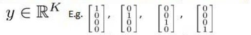
$J(\Theta)=-\frac{1}{m}\sum_{i=1}^{m}\sum_{k=1}^{K}[y^{(i)}_k(log(h_\Theta(x^{(i)}))_k)+(1-y^{(i)}_k)log(1-(h_{\Theta}(x^{(i)}))_k)]$
$+\frac{\lambda }{2m}\sum_{l=1}^{L-1}\sum_{i=1}^{s_l}\sum_{j=1}^{s_l+1}(\Theta_{ji}^{l})^{2}$
注意:$(h_\Theta(x^{(i)}))_k=a^{(3)}_k$,第k个输出单元。
该代价函数正则化时忽略偏差项,最里层的循环$𝑗$循环所有的行由$𝑠^{𝑙 +1}$ 层的激活单元数决定),循环$𝑖$则循环所有的列,由该层($𝑠^{𝑙}$层)的激活单元数所决定。
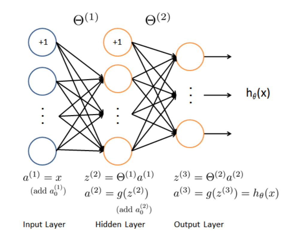
神经网络跟之前我们学过的逻辑回归思想差不多。在这里我们的神经网络有三层(输入层,隐藏层,输出层)。
1,我们先随机初始化参数$\Theta1$与$\Theta2$(已添加偏差项)。
function W = randInitializeWeights(L_in, L_out)
%RANDINITIALIZEWEIGHTS Randomly initialize the weights of a layer with L_in
%incoming connections and L_out outgoing connections
%   W = RANDINITIALIZEWEIGHTS(L_in, L_out) randomly initializes the weights
%   of a layer with L_in incoming connections and L_out outgoing
%   connections.
%
%   Note that W should be set to a matrix of size(L_out, 1 + L_in) as
%   the first column of W handles the "bias" terms
%

% You need to return the following variables correctly
W = zeros(L_out, 1 + L_in);

% ====================== YOUR CODE HERE ======================
% Instructions: Initialize W randomly so that we break the symmetry while
%               training the neural network.
%
% Note: The first column of W corresponds to the parameters for the bias unit
%


##epsilon_init=sqrt(6)/(sqrt(L_in+L_out));
epsilon_init=0.12;
W=rand(L_out,1+L_in)*2*epsilon_init-epsilon_init;


% =========================================================================

end
2,我们有了参数$\Theta$,我们就可以使用前向传播去计算$h_{\Theta}(x)$,这跟之前的逻辑回归差不多
3,紧接着我们要求代价函数的偏导数$\frac{\partial }{\partial \Theta^{(l)}_{ij}}J(\Theta)$(𝑖 代表下一层中误差单元的下标,𝑗 代表目前计算层中的激活单元的下标),
在这里我们采用一种叫做反向传播(Backpropagation)来计算偏导数,完成梯度下降。
反向传播:对于每一个样例,都使用以下四步
3-1:先使用前向传播计算$a^{l}$,$l=1,2,...,L$
3-2: 从最后一层的误差$\delta$开始计算,$\delta^{(L)}=a^{(L)}-y$,
在这,即:$\delta^{(3)}=a^{(3)}-y$
3-3: 紧接着计算隐藏层$\delta^{(l)}$,$\delta^{(l)}=(\Theta^{(l)})^{T}\delta^{(l+1)}.*{g}'(z^{(l)})$,
${g}'(z^{(l)})=g(z^{(l)}).*(1-g(z^{(l)}))$
Sigmoid gradient求导代码:
function g = sigmoidGradient(z)
%SIGMOIDGRADIENT returns the gradient of the sigmoid function
%evaluated at z
%   g = SIGMOIDGRADIENT(z) computes the gradient of the sigmoid function
%   evaluated at z. This should work regardless if z is a matrix or a
%   vector. In particular, if z is a vector or matrix, you should return
%   the gradient for each element.

g = zeros(size(z));

% ====================== YOUR CODE HERE ======================
% Instructions: Compute the gradient of the sigmoid function evaluated at
%               each value of z (z can be a matrix, vector or scalar).

g=sigmoid(z).*(1-sigmoid(z));

% =============================================================


end
在这,即:$\delta^{(2)}=(\Theta^{(2)})^{T}\delta^{(3)}.*{g}'(z^{(2)})$ (除开偏差项)
3-4:使用以下公式来实现累积梯度,这跟前面的逻辑回归差不多,也是累加所有样例的梯度后更新。
$\Delta ^{(l)}:=\Delta ^{(l)}+\delta^{(l+1)}(a^{(l)})^{T}$
最后:$\frac{\partial }{\partial \Theta^{(l)}_{ij}}J(\Theta)=D^{(l)}_{ij}=\frac{1}{m}\Delta^{(l)}_{ij}$ ,$j=0$
$\frac{\partial }{\partial \Theta^{(l)}_{ij}}J(\Theta)=D^{(l)}_{ij}=\frac{1}{m}\Delta^{(l)}_{ij}+ \frac{\lambda}{m}\Theta^{(l)}_{ij}$,$j \geq 1$
代价函数以及反向传播代码:
function [J grad] = nnCostFunction(nn_params, ...
                                   input_layer_size, ...
                                   hidden_layer_size, ...
                                   num_labels, ...
                                   X, y, lambda)
%NNCOSTFUNCTION Implements the neural network cost function for a two layer
%neural network which performs classification
%   [J grad] = NNCOSTFUNCTON(nn_params, hidden_layer_size, num_labels, ...
%   X, y, lambda) computes the cost and gradient of the neural network. The
%   parameters for the neural network are "unrolled" into the vector
%   nn_params and need to be converted back into the weight matrices.
%
%   The returned parameter grad should be a "unrolled" vector of the
%   partial derivatives of the neural network.
%

% Reshape nn_params back into the parameters Theta1 and Theta2, the weight matrices
% for our 2 layer neural network

%还原Theta1与Theta2
Theta1 = reshape(nn_params(1:hidden_layer_size * (input_layer_size + 1)), ...
                 hidden_layer_size, (input_layer_size + 1));

Theta2 = reshape(nn_params((1 + (hidden_layer_size * (input_layer_size + 1))):end), ...
                 num_labels, (hidden_layer_size + 1));

% Setup some useful variables
m = size(X, 1);

% You need to return the following variables correctly
J = 0;
Theta1_grad = zeros(size(Theta1)); %梯度下降的偏导数1
Theta2_grad = zeros(size(Theta2)); %梯度下降的偏导数2

% ====================== YOUR CODE HERE ======================
% Instructions: You should complete the code by working through the
%               following parts.
%
% Part 1: Feedforward the neural network and return the cost in the
%         variable J. After implementing Part 1, you can verify that your
%         cost function computation is correct by verifying the cost
%         computed in ex4.m
%
% Part 2: Implement the backpropagation algorithm to compute the gradients
%         Theta1_grad and Theta2_grad. You should return the partial derivatives of
%         the cost function with respect to Theta1 and Theta2 in Theta1_grad and
%         Theta2_grad, respectively. After implementing Part 2, you can check
%         that your implementation is correct by running checkNNGradients
%
%         Note: The vector y passed into the function is a vector of labels
%               containing values from 1..K. You need to map this vector into a
%               binary vector of 1's and 0's to be used with the neural network
%               cost function.
%
%         Hint: We recommend implementing backpropagation using a for-loop
%               over the training examples if you are implementing it for the
%               first time.
%
% Part 3: Implement regularization with the cost function and gradients.
%
%         Hint: You can implement this around the code for
%               backpropagation. That is, you can compute the gradients for
%               the regularization separately and then add them to Theta1_grad
%               and Theta2_grad from Part 2.
%


  % 根据已给的参数Θ(1)和Θ(2),使用前向传播算法算出hθ(x),维度为10
  a1=[ones(m,1) X];
  a2=sigmoid(a1*Theta1');
  a2=[ones(m,1) a2];
  h=sigmoid(a2*Theta2'); %5000x10

  yk=zeros(m,num_labels); %定义5000x10的训练集输出向量

  %根据数据集y给yk向量赋值
  for i=1:m
      yk(i,y(i))=1;
  endfor

  %前向传播代价函数,忽略正则化,该代价函数就为矩阵h与矩阵yk点乘后计算总和
  J=(1/m)*sum(sum((-yk.*log(h)-(1-yk).*log(1-h))));


   item1=Theta1;
   item1(:,1)=0;
   item2=Theta2;
   item2(:,1)=0;
   %加上正则化
  J=J+lambda/2/m*(sum(sum(power(item1,2)))+sum(sum(power(item2,2))));


  %反向传播
  for t=1:m %对于每一个样例,都计算一次该样例每个参数的偏导数

    a1=X(t,:);
    a1=[1 a1]'; %1x401
    z2=Theta1*a1; %25x1
    a2=[1;sigmoid(z2)]; %26x1
    z3=Theta2*a2;
    a3=sigmoid(z3); %10x1
    y=yk(t,:); %1x10
    delta3=a3-y'; %10x1
    delta2=Theta2(:,2:end)'*delta3.*sigmoidGradient(z2); %25x1
    Theta1_grad=Theta1_grad+delta2*a1'; %25x401 %累加梯度
    Theta2_grad=Theta2_grad+delta3*a2';  %10x26

  end

  %梯度总和除以m
  Theta1_grad=Theta1_grad./m;
  Theta2_grad=Theta2_grad./m;


  %梯度正则化
  Theta1(:,1)=0;
  Theta2(:,1)=0;
  Theta1_grad=Theta1_grad+(lambda/m).*Theta1;
  Theta2_grad=Theta2_grad+(lambda/m).*Theta2;


% -------------------------------------------------------------

% =========================================================================

% Unroll gradients
%展开合并为一个大的列向量
grad = [Theta1_grad(:) ; Theta2_grad(:)];


end
4,在我们写好代价函数以及梯度下降的模型时,我们要先进行梯度的数值检验(Numerical Gradient Checking),也就是我们先在一个小样本中测验,如果通过了测试,我们就使用大规模的数据去跑神经网络,这样能更好的求最优解。
当𝜃是一个向量时,我们则需要对偏导数进行检验。因为代价函数的偏导数检验只针对 一个参数的改变进行检验,下面是一个只针对𝜃1进行检验的示例:
$\frac{\partial }{\partial \Theta_{1}}=\frac{J((\theta_1+\epsilon),\theta_2,\theta_3,...,\theta_n)-J((\theta_1-\epsilon),\theta_2,\theta_3,...,\theta_n)}{2\epsilon }$
最后我们还需要对通过反向传播方法计算出的偏导数进行检验,检验时,我们要将该矩阵展开 成为向量,同时我们也将 𝜃 矩阵展开为向量
5,最后我们调用预测函数,求的神经网络的预测准确率为95%左右,要是我们迭代次数更多,预测准确率会更高。
总结: 神经网络是非常强大的模型,可以形成高度复杂的决策边界。
训练神经网络:
1. 参数的随机初始化
2. 利用正向传播方法计算所有的 $h_{\theta}(x)$
3. 编写计算代价函数 J 的代码
4. 利用反向传播方法计算所有偏导数
5. 利用数值检验方法检验这些偏导数
6. 使用优化算法(fmincg)来最小化代价函数
我的便签:做个有情怀的程序员。

 浙公网安备 33010602011771号