[Python & Machine Learning] 学习笔记之scikit-learn机器学习库

1. scikit-learn介绍

　　scikit-learn是Python的一个开源机器学习模块，它建立在NumPy，SciPy和matplotlib模块之上。值得一提的是，scikit-learn最先是由David Cournapeau在2007年发起的一个Google Summer of Code项目，从那时起这个项目就已经拥有很多的贡献者了，而且该项目目前为止也是由一个志愿者团队在维护着。

　　scikit-learn最大的特点就是，为用户提供各种机器学习算法接口，可以让用户简单、高效地进行数据挖掘和数据分析。

　　scikit-learn主页：scikit-learn homepage

2. scikit-learn安装

　　scikit-learn的安装方法有很多种，而且也是适用于各种主流操作系统，scikit-learn主页上也分别详细地介绍了在不同操作系统下的三种安装方法，具体安装详情请移步至 installing scikit-learn。

　　在这里，首先向大家推荐一款学习Python的强大的开发环境python(x,y)。python(x,y)是一个基于python的科学计算软件包，它包含集成开发环境Eclipse和Python开发插件pydev、数据交互式编辑和可视化工具spyder，而且还内嵌了Python的基础数据库numpy和高级数学库scipy、3D可视化工具集MayaVi、Python界面开发库PyQt、Python与C/C++混合编译器SWIG。除此之外，python(x,y)配备了丰富齐全的帮助文档，非常方便科研人员使用。

　　对于像楼主这样，在学校习惯了用Matlab仿真搞科研的学生而言，python(x,y)是学习Python的一个绝佳选择，其中内嵌的spyder提供了类似于Matlab的交互界面，可以很方便地使用。python(x,y)的下载请点击这里：python(x,y)下载。

　　由于scikit-learn是基于NumPy、SciPy和matplotlib模块的，所以在安装scikit-learn之前必须要安装这3个模块，这就很麻烦。但是，如果你提前像楼主这样安装了python(x,y)，它本身已经包含上述的模块，你只需下载与你匹配的scikit-learn版本，直接点击安装即可。

　　scikit-learn各种版本下载：scikit-learn下载。

3. scikit-learn载入数据集

　　scikit-learn内包含了常用的机器学习数据集，比如做分类的iris和digit数据集，用于回归的经典数据集Boston house prices。

　　scikit-learn载入数据集实例：

from sklearn import datasets
iris = datasets.load_iris()

　　scikit-learn载入的数据集是以类似于字典的形式存放的，该对象中包含了所有有关该数据的数据信息（甚至还有参考文献）。其中的数据值统一存放在.data的成员中，比如我们要将iris数据显示出来，只需显示iris的data成员：

print iris.data

　　数据都是以n维（n个特征）矩阵形式存放和展现，iris数据中每个实例有4维特征，分别为：sepal length、sepal width、petal length和petal width。显示iris数据：

[[ 5.1  3.5  1.4  0.2]
 [ 4.9  3.   1.4  0.2]
　　　　... ...
 [ 5.9  3.   5.1  1.8]]

　　如果是对于监督学习，比如分类问题，数据中会包含对应的分类结果，其存在.target成员中：

print iris.target

　　对于iris数据而言，就是各个实例的分类结果：

[0, 0, 0, 0, 0, 0, 0, 0, 0, 0, 0, 0, 0, 0, 0, 0, 0, 0, 0, 0, 0, 0, 0,
 0, 0, 0, 0, 0, 0, 0, 0, 0, 0, 0, 0, 0, 0, 0, 0, 0, 0, 0, 0, 0, 0, 0,
 0, 0, 0, 0, 1, 1, 1, 1, 1, 1, 1, 1, 1, 1, 1, 1, 1, 1, 1, 1, 1, 1, 1,
 1, 1, 1, 1, 1, 1, 1, 1, 1, 1, 1, 1, 1, 1, 1, 1, 1, 1, 1, 1, 1, 1, 1,
 1, 1, 1, 1, 1, 1, 1, 1, 2, 2, 2, 2, 2, 2, 2, 2, 2, 2, 2, 2, 2, 2, 2,
 2, 2, 2, 2, 2, 2, 2, 2, 2, 2, 2, 2, 2, 2, 2, 2, 2, 2, 2, 2, 2, 2, 2,
 2, 2, 2, 2, 2, 2, 2, 2, 2, 2, 2, 2]

4. scikit-learn学习和预测

　　scikit-learn提供了各种机器学习算法的接口，允许用户可以很方便地使用。每个算法的调用就像一个黑箱，对于用户来说，我们只需要根据自己的需求，设置相应的参数。

　　比如，调用最常用的支撑向量分类机（SVC）：

from sklearn import svm
clf = svm.SVC(gamma=0.001, C=100.) #不希望使用默认参数，使用用户自己给定的参数
print clf

　　分类器的具体信息和参数：

SVC(C=100.0, cache_size=200, class_weight=None, coef0=0.0, degree=3,
    gamma=0.001, kernel='rbf', max_iter=-1, probability=False,
    random_state=None, shrinking=True, tol=0.001, verbose=False)

　　分类器的学习和预测可以分别利用 fit(X,Y) 和 predict(T) 来实现。

　　例如，将digit数据划分为训练集和测试集，前n-1个实例为训练集，最后一个为测试集（这里只是举例说明fit和predict函数的使用）。然后利用fit和predict分别完成学习和预测，代码如下：

from sklearn import datasets
from sklearn import svm
clf = svm.SVC(gamma=0.001, C=100.)
digits = datasets.load_digits()
clf.fit(digits.data[:-1], digits.target[:-1])
result=clf.predict(digits.data[-1])
print result

　　预测结果为：[8]

　　我们可以通过程序来查看测试集中的手写体实例到底长什么样来简单验证一下分类效果，代码和结果如下所示：

import matplotlib.pyplot as plot
plot.figure(1, figsize=(3, 3))
plot.imshow(digits.images[-1], cmap=plot.cm.gray_r, interpolation='nearest')
plot.show()

　　最后一个手写体实例为：

　　

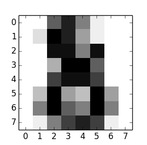
　　我们可以看到，这就是一个手写的数字“8”的，实际上正确的分类也是“8”。我们通过这个简单的例子，就是为了简单的学习如何来使用scikit-learn来解决分类问题，实际上这个问题要复杂得多。（PS：学习就是循序渐进，弄懂一个例子，就会弄懂第二个，... ，然后就是第n个，最后就会形成自己的知识和理论，你就可以轻松掌握，来解决各种遇到的复杂问题。）

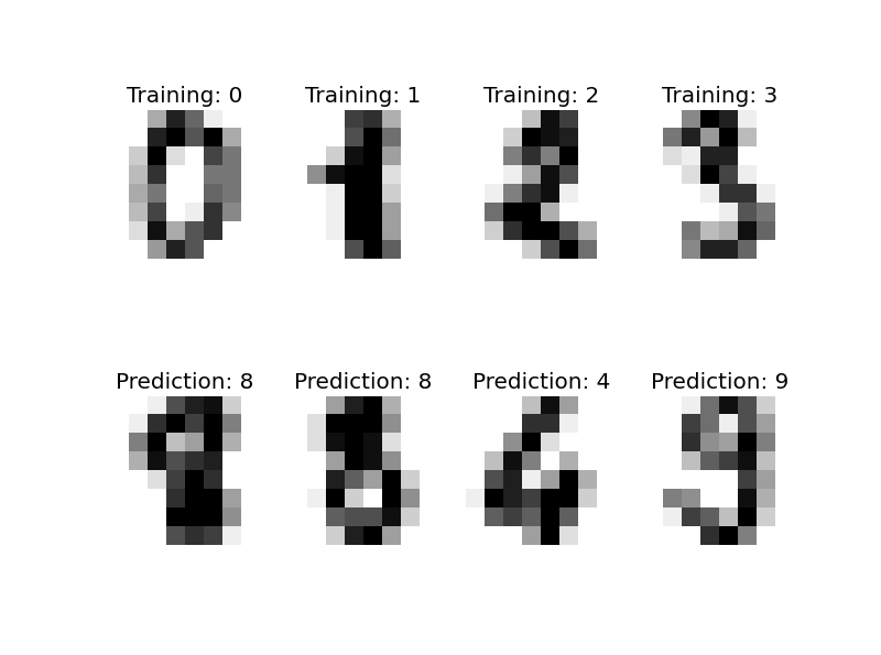
　　再为各位展示一个scikit-learn解决digit分类（手写体识别）的程序（by Gael Varoquaux），相信看过这个程序大家一定会对scikit-learn机器学习库有了一定的了解和认识。

import matplotlib.pyplot as plt

# Import datasets, classifiers and performance metrics
from sklearn import datasets, svm, metrics

# The digits dataset
digits = datasets.load_digits()

# The data that we are interested in is made of 8x8 images of digits, let's
# have a look at the first 3 images, stored in the `images` attribute of the
# dataset.  If we were working from image files, we could load them using
# pylab.imread.  Note that each image must have the same size. For these
# images, we know which digit they represent: it is given in the 'target' of
# the dataset.
images_and_labels = list(zip(digits.images, digits.target))
for index, (image, label) in enumerate(images_and_labels[:4]):
    plt.subplot(2, 4, index + 1)
    plt.axis('off')
    plt.imshow(image, cmap=plt.cm.gray_r, interpolation='nearest')
    plt.title('Training: %i' % label)

# To apply a classifier on this data, we need to flatten the image, to
# turn the data in a (samples, feature) matrix:
n_samples = len(digits.images)
data = digits.images.reshape((n_samples, -1))

# Create a classifier: a support vector classifier
classifier = svm.SVC(gamma=0.001)

# We learn the digits on the first half of the digits
classifier.fit(data[:n_samples / 2], digits.target[:n_samples / 2])

# Now predict the value of the digit on the second half:
expected = digits.target[n_samples / 2:]
predicted = classifier.predict(data[n_samples / 2:])

print("Classification report for classifier %s:\n%s\n"
      % (classifier, metrics.classification_report(expected, predicted)))
print("Confusion matrix:\n%s" % metrics.confusion_matrix(expected, predicted))

images_and_predictions = list(zip(digits.images[n_samples / 2:], predicted))
for index, (image, prediction) in enumerate(images_and_predictions[:4]):
    plt.subplot(2, 4, index + 5)
    plt.axis('off')
    plt.imshow(image, cmap=plt.cm.gray_r, interpolation='nearest')
    plt.title('Prediction: %i' % prediction)

plt.show()

　　输出结果：

Classification report for classifier SVC(C=1.0, cache_size=200, class_weight=None, coef0=0.0, degree=3,
  gamma=0.001, kernel='rbf', max_iter=-1, probability=False,
  random_state=None, shrinking=True, tol=0.001, verbose=False):
             precision    recall  f1-score   support

          0       1.00      0.99      0.99        88
          1       0.99      0.97      0.98        91
          2       0.99      0.99      0.99        86
          3       0.98      0.87      0.92        91
          4       0.99      0.96      0.97        92
          5       0.95      0.97      0.96        91
          6       0.99      0.99      0.99        91
          7       0.96      0.99      0.97        89
          8       0.94      1.00      0.97        88
          9       0.93      0.98      0.95        92

avg / total       0.97      0.97      0.97       899


Confusion matrix:
[[87  0  0  0  1  0  0  0  0  0]
 [ 0 88  1  0  0  0  0  0  1  1]
 [ 0  0 85  1  0  0  0  0  0  0]
 [ 0  0  0 79  0  3  0  4  5  0]
 [ 0  0  0  0 88  0  0  0  0  4]
 [ 0  0  0  0  0 88  1  0  0  2]
 [ 0  1  0  0  0  0 90  0  0  0]
 [ 0  0  0  0  0  1  0 88  0  0]
 [ 0  0  0  0  0  0  0  0 88  0]
 [ 0  0  0  1  0  1  0  0  0 90]]

　　

5. 总结

　　1）scikit-learn的介绍和安装；

　　2）对scikit-learn有个概括的了解，能够尝试利用scikit-learn来进行数据挖掘和分析。

6. 参考内容

　　[1] An introduction to machine learning with scikit-learn

　　 [2] 机器学习实战