
Reference : Lucas-Kanade 20 Years On: A Unifying Framework
---对原文进行了简单翻译
Abstract.
由于Lucas Kanade算法在1981年图像对准时提出,已经成为在计算机视觉中最常用的技术。应用范围从光流跟踪到分层运动,拼接技术和面部编码。已经提出了许多算法,并对原始公式进行了多种扩展。我们概述了图像对齐,描述了大多数算法及其在一致框架中的扩展。我们专注于逆合成算法,也是最近提出的一个有效的算法。我们研究哪些Lucas Kanade的扩展可以用于逆向合成算法没有显著的效率损失,哪些不能。
1.Introduction
图像对齐包括移动和可能形变,以尽量减少样板和图像之间的差异。自从在Lucas Kanade光流算法第一次使用图像对齐 (Lucas and Kanade, 1981), 图像对齐已成为计算机视觉技术应用最为广泛。除了光流,它的一些其他应用包括跟踪 (Black and Jepson, 1998; Hager and Belhumeur, 1998), 参数化和分层运动估计 (Bergen et al., 1992), 拼接技术 (Shum and Szeliski, 2000), 医学图像配准 (Christensen and Johnson, 2001),和面部编码 (Baker and Matthews, 2001; Cootes et al., 1998).
通常的图像对齐方法是梯度下降。其他多种数值算法例如差异分解 (Gleicher, 1997)和线性回归 (Cootes et al., 1998)也已提出,但梯度下降是实际的标准。虽然梯度下降可以在各种不同的方式中执行,但各种方法之间的其中一个区别是:它们是否估计参数的加性增量 (the additive approach (Lucas and Kanade, 1981)), 或者它们是否估计增量的偏移,然后由偏移的当前估计组成 (the compositional approach (Shum and Szeliski, 2000)). 另一个区别是算法是否在每个梯度下降步骤中执行高斯牛顿、牛顿、最速下降或Levenberg Marquardt近似。
我们提出了一个统一的图像对齐框架,以一致的方式描述各种算法及其扩展。在框架中,我们专注于逆向合成算法,并且提出了一个高效的算法(Baker and Matthews, 2001)。我们研究哪些扩展Lucas Kanade可以应用于逆向组合算法的效率没有显著的效率损失,哪些扩展需要额外的计算。在可能的情况下,我们提供实证结果来说明各种算法及其扩展。
补充:预备知识---
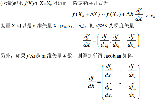
[1].泰勒展开
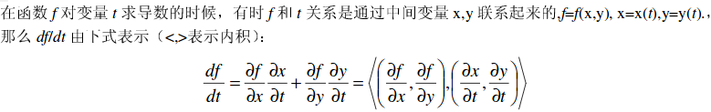
[2].复合函数链式求导法则
2.Background: Lucas-Kanade(加性算法)
初始的图像对齐算法是Lucas-Kanade algorithm (Lucas and Kanade, 1981),目的是用一组参数p从一个图像区域(patch)采样 与模板图像
与模板图像 进行匹配,使得误差最小。
其中, 是包含像素坐标的列向量,
 参数向量,
参数向量, 表示为image warping ,实际上可以理解为坐标变换,以决定在图像上的采样点。
变换是在模板图像 的坐标系中取像素
 ,并将其映射到图像
 坐标系中的亚像素位置。
这个公式需要说明:
- 2个参数表示位移,偏差为:
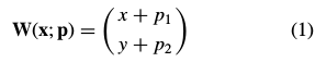 ,其中
,其中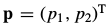 ,这就是一般的光流法。
 - 如果我们跟踪的图像块移动比较大,我们可以考虑仿射形变的设置--- 6个参数的仿射变换,需要至少3个对应点。
 ,即
,即

- 4个参数的相似变换只表达变比和旋转,需要至少2个对应点(如下)。

- P也可以是8个参数表达的透射变换。
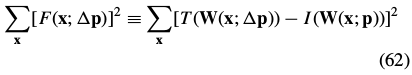
2.1.Goal of the Lucas-Kanade Algorithm
给定一个模板 和一个输入
和一个输入 ,以及一个或多个变换
 ,求一个参数最佳的变换
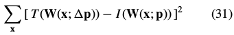
 ,使得两个图像之间的误差平方和最小化:
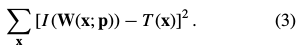
在求最优解的时候,该算法假设目前的变换参数 已知,并迭代的计算的增量
 ,使得更新后的能令上式比原来更小。则上式改写为:
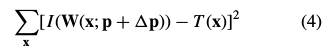
通过 ,每次更新参数:
这两个步骤迭代直到估计参数收敛。收敛性检验是向量的某个范数是否低于阈值 .
. 
|
算法流程: 1.初始化参数向量 2.计算 3.更新 4.若 |
 及其关于
及其关于
2.2.Derivation of the Lucas-Kanade Algorithm 推导
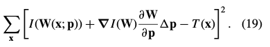
Lucas-Kanade算法(一个基于梯度下降高斯牛顿非线性优化算法)。对 做一阶泰勒级数展开线性近似,则目标函数变为:
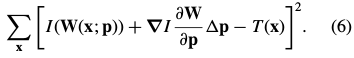
其中![]()
其中, 表示在图像
表示在图像![]() 的图像梯度。
的图像梯度。 是warp变换的雅克比。
 为最速下降图像(See Section 4.3 )。注意:这里的求和下标x为patch。
如果![]() ---
--- 是二维坐标,也就是说每行是
 中每个分量对于的每个参数分量的导数:

|
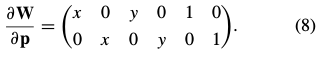
例如,(2)的仿射变换的雅克比:
对于patch 上的每个点: |

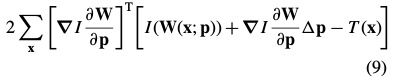
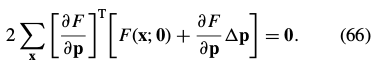
对(6)求导[复合函数求导],得到下式:
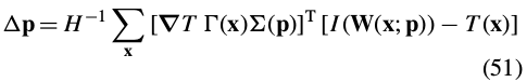
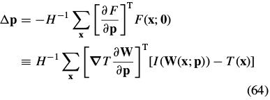
将表达式(9)设为零,并求出表达式(6)最小值的解析解:
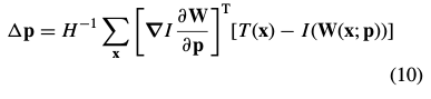
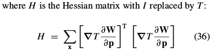
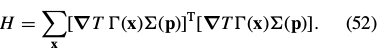
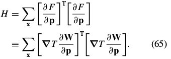
其中, 是n×n(高斯牛顿近似) Hessian 矩阵:
可参考:http://image.sciencenet.cn/olddata/kexue.com.cn/upload/blog/file/2010/9/2010929122517964628.pdf
流程过程:
|
1) 利用
2) 计算
3) 计算 4) 计算在 5) 计算最速梯度下降图
6) 利用上述公式计算Hessian矩阵
7) 利用上面步骤计算得到的值,计算
8) 利用上述提到的公式计算参数向量的增量
9) 更新
|


 ,将
,将 的坐标对应到
 的坐标,得到
 。即
。即 ,获得误差图像。
 设定下的
设定下的 (即代入当前参数
 ,计算
,计算 (即利用
(即利用


2.3.Requirements on the Set of Warps
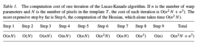
2.4.Computational Cost of the Lucas-Kanade Algorithm
3.2. Inverse Compositional Image Alignment(逆向组合算法)
3.2.1. Goal of the Inverse Compositional Algorithm
The inverse compositional algorithm minimizes:
with respect to  (note that the roles of
  and
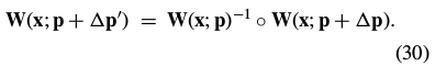
and  are reversed交换了) and then updates the warp:

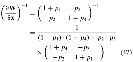
the inverse of the affine warp in Eq. (2) :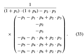 |
If , the affine warp is degenerate(变质的) and not invertible.All pixels are mapped onto a straight line in
  . We exclude all such affine warps from consideration.
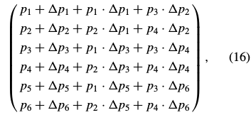
The set of all such affine warps is then still closed under composition, as can be seen by computing  for the parameters in Eq. (16). After considerable simplification, this value becomes
  ·
· which can only equal zero if one of the two warps being composed is degenerate.
3.2.2. Derivation of the Inverse Compositional
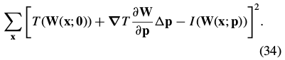
式(31)进行一阶泰勒展开:
Assuming again without loss of generality that W(x; 0) is the identity(恒等) warp, the solution to this least-squares problem is:

预处理: 1) 计算模板 2) 计算在 3) 计算最速梯度下降图 4) 利用公式计算Hessian矩阵
迭代: 5) 利用 6) 计算 7) 利用上面步骤计算得到的值,计算 8) 利用上述提到的公式计算参数向量的增量 9) 更新 |

 设定下的
设定下的
 。即利用
。即利用


 。即将原有
。即将原有 矩阵的逆相乘。
3.2.3. Requirements on the Set of Warps.
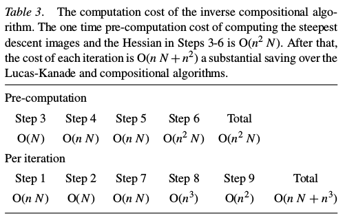
3.2.4. Computational Cost of the Inverse Compositional Algorithm.
3.The Quantity Approximated and the Warp Update Rule
以上并不是唯一的方法最小化表达式,在这一部分中我们列出了3个可供选择的方法,都可证明等价于Lucas Kanade算法。
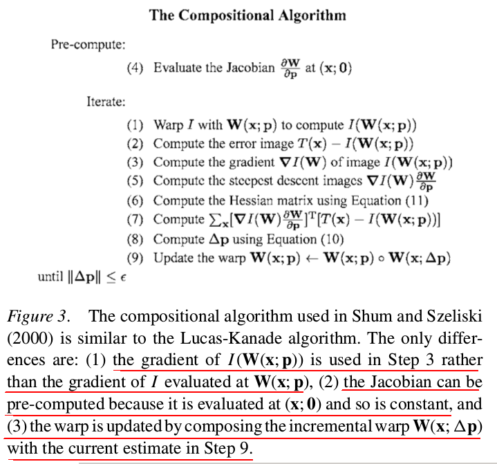
3.1.Compositional Image Alignment 组合图像对齐(前向组合算法)
3.1.1. Goal of the Compositional Algorithm.
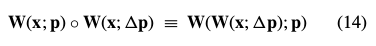
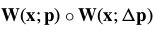
合成算法,最著名的就是Shum and Szeliski (2000), 近似最小化:
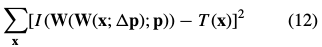
关于每次迭代中的,然后更新变换(warp)为:

合成方法迭代通过一个增量的变换 ,而不是用参数
 的添加更新。
在Lucas Kanade算法的公式(4)和(5)添加的方法与公式(12)和(13)合成的方法来对比,被证明是等价的,为一阶泰勒偏导:
|
对应于公式(2):
一个简单双线性的 |

 和
和 的参数组合。
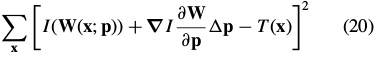
3.1.2. Derivation of the Compositional Algorithm.推导
我们将公式(12)进行一阶泰勒展开:

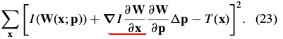
In this expression denotes the warped image
 . It is possible to further expand:

我们假设 是恒等变形,即
 ,式(17)简化为:
|
|
3.1.3. Requirements on the Set of Warps.
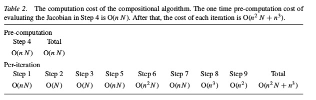
3.1.4. Computational Cost of the Compositional Algorithm.
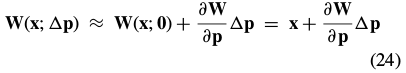
3.1.5. Equivalence of the Additive and Compositional Algorithms. 加法与合成的等价性
In the additive formulation in Eq. (6) we minimize:
with respect to and then update
  .The corresponding update to the warp is(通过一阶泰勒展开):

In the compositional formulation in Eq. (19) we minimize:

using Eq. (18), simplifies to:
In the compositional approach, the update to the warp is  . 对
. 对 进行一阶泰勒展开:

Combining these last two equations, and applying the Taylor expansion again, gives the update in the compositional formulation as:
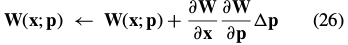
From Eq. (21) we see that the first of these expressions:
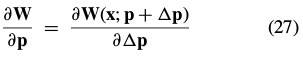
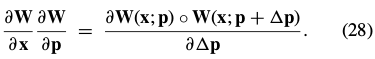
and from Eq. (26) we see that the second of these expressions:
if (there is an  > 0 such that) for any
  (
(  ) there is a
  such that:

This condition means that the function between and is defined in both directions. The expressions in Eq. (27) and (28) therefore span(跨越) the same linear space.
If the warp is invertible Eq. (29) always holds since can be chosen such that:
In summary, if the warps are invertible(可逆)then the two formulations are equivalent. In Section 3.1.3, above, we stated that the set of warps must form a semi-group(半群) for the compositional algorithm to be applied.While this is true, for the compositional algorithm also to be provably equivalent to the Lucas-Kanade algorithm, the set of warps must form a group; i.e. every warp must be invertible.
3.3.Inverse Additive Image Alignment(逆加性算法)
3.3.1. Goal of the Inverse Additive Algorithm.
An image alignment algorithm that addresses this difficulty is the Hager-Belhumeur algorithm (Hager and Belhumeur, 1998). Although the derivation in Hager and Belhumeur (1998) is slightly different from the
derivation(推导) in Section 3.2.5, the Hager-Belhumeur algorithm does fit into our framework as an inverse additive algorithm.
The initial goal of the Hager-Belhumeur algorithm is the same as the Lucas-Kanade algorithm;i.e. to minimize  with respect to
  and then update the parameters
  ←
← . Rather than changing variables like in Section 3.2.5, the roles of the template and the image are switched(切换) as follows. First the Taylor expansion is performed, just as in Section 2.1:

The template and the image are then switched by deriving the relationship between  and
and  .
.
In Hager and Belhumeur (1998) it is assumed that the current estimates of the parameters are approximately correct:

This is equivalent to the assumption we made in Section 3.2.5 that  is
is  . Taking partial derivatives(偏导数) with respect to
  and using the chain rule (链规则) gives:
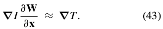
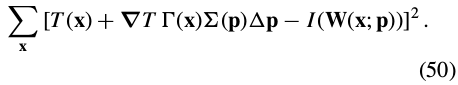
将式(43)变形,带入(41)中:
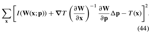
To completely change the role of the template and the image  , we replace with
  . The final goal of the Hager-Belhumeur algorithm is then to iteratively solve:
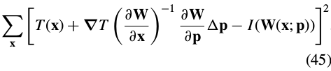
and update the parameters  .
.
3.3.2. Derivation of the Inverse Additive Algorithm.
To derive an efficient inverse additive algorithm, Hager and Belhumeur assumed that the warp  has a particular form. They assumed that the product of the two Jacobians can be written as:

 is a
is a  matrix that is just a function of the template coordinates and
  is a
is a  matrix that is just a function of the warp parameters (and where k is 正整数.)
Not all warps can be written in this form, but some can;
|
e.g. if W is the affine warp of Eq. (2):
Since diagonal matrices commute with any other matrix,and since the 2 × 6 matrix
|


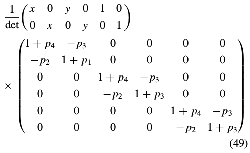
Equation (45) can then be re-written as:
Equation (50) has the closed form solution:
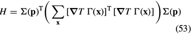
Since  does not depend upon(依赖于)
 , the Hessian can be re-written as:
令
则

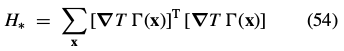
Inserting this expression into Eq. (51) and simplifying yields:
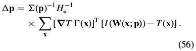
Equation (56) can be split into two steps:
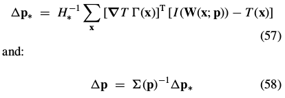
where nothing in the first step depends on the current estimate of the warp parameters  . The Hager-Belhumeur algorithm consists of iterating applying Eq. (57) and then updating the parameters
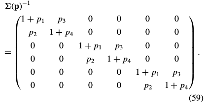
|
For the affine warp of Eq. (2): |

3.3.3. Requirements on the Set of Warps.
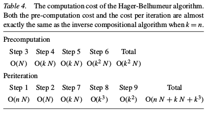
3.3.4. Computational Cost of the Inverse Additive Algorithm.
3.3.5. Equivalence of the Inverse Additive and Compositional Algorithms for Affine Warps.
3.4.Empirical Validation实验验证
3.5. Summary
4.The Gradient Descent Approximation梯度下降近似
4.1.The Gauss-Newton Algorithm
The Gauss-Newton inverse compositional algorithm attempts to minimize Eq. (31):
 一阶泰勒展开:

对上式 求导=0:
求导=0:
 、
、
求解得:
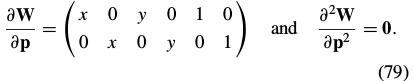
4.2. The Newton Algorithm


二阶泰勒展开:
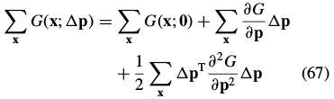
其中:
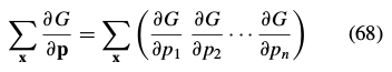 是
是 的梯度。
的梯度。
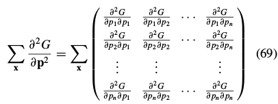 是的Hessian矩阵。
4.2.1. Relationship with the Hessian in the Gauss-Newton Algorithm.

Comparing Eqs. (67) and (70):
the gradient is 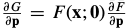
the Hessian is approximated: 
这个近似是一个一阶近似,在这个意义上,它是G的Hessian的近似。 F的Hessian在近似中被忽略。G的Hessian的充分表达式是:

4.2.2. Derivation of the Gradient and the Hessian.
If  then the gradient is:
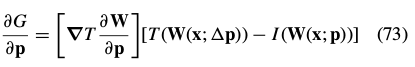
The Hessian:
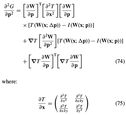 是模板T的二阶导数的矩阵???

Equations (73) and (74) hold for arbitrary  . In the Newton algorithm, we just need their values at
  . When
  , the gradient simplifies to:

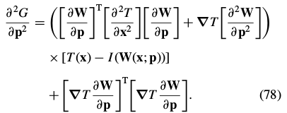
These expressions depend on the Jacobian  and the Hessian
  of the warp.
|
For the affine warp of Eq. (2) these values are:
|
4.2.3. Derivation of the Newton Algorithm.
The derivation of the Newton algorithm begins with Eq. (67), the second order approximation(二阶近似) to .
Differentiating this expression with respect to and equating the result with zero yields (Gill et al., 1986; Press et al., 1992):
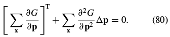
The minimum is then attained at:
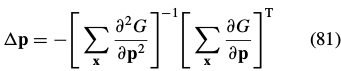
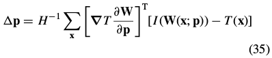
where the gradient and the Hessian are given in Eqs. (77) and (78). Ignoring the sign change and the transpose, Eqs. (77), (78), and (81) are almost identical(相等) to Eqs. (35) and (36) in the description of the
inverse compositional algorithm in Section 3.2. The only difference is the second order term (the first term) in the Hessian in Eq. (78); if this term is dropped the
4.2.4. Computational Cost of the Newton Inverse Compositional Algorithm
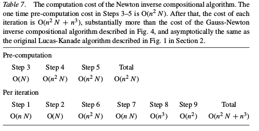
Figure 1. The Lucas-Kanade algorithm (Lucas and Kanade, 1981)
Figure 2. A schematic overview of the Lucas-Kanade algorithm (Lucas and Kanade, 1981).
Figure 3. The compositional algorithm used in Shum and Szeliski (2000) is similar to the Lucas-Kanade algorithm.
Figure 4. The inverse compositional algorithm (Baker and Matthews, 2001) is derived from the forwards compositional algorithm by inverting the roles of I and T similarly to the approach in Hager and Belhumeur (1998).
Figure 5. The Hager-Belhumeur inverse additive algorithm (Hager and Belhumeur, 1998) is very similar to the inverse compositional algorithm in Fig. 4.
Figure 6. Examples of the four algorithms converging.
Figure 7. The average rates of convergence computed over a large number of randomly generated warps.
Figure 8. The average frequency of convergence computed over a large number of randomly generated warps.
Figure 9. The average rates of convergence and average frequencies of convergence for the affine warp for three different images: “Simon” (an image of the face of the first author), “Knee” (an image of an x-ray of a knee), and “Car” (an image of car.)
Figure 10. The effect of intensity noise on the rate of convergence and the frequency of convergence for affine warps. //
Figure 11. Compared to the Gauss-Newton inverse compositional algorithm in Fig. 4, the Newton inverse compositional algorithm is considerably more complex.
Table 1. The computation cost of one iteration of the Lucas-Kanade algorithm.
Table 2. The computation cost of the compositional algorithm.
Table 3. The computation cost of the inverse compositional algorithm.
Table 4. The computation cost of the Hager-Belhumeur algorithm.(inverse additive algorithm)
Table 5. Timing results for our Matlab implementation of the four algorithms in milliseconds.
able 6. A framework for gradient descent image alignment algorithms.//
Table 7. The computation cost of the Newton inverse compositional algorithm.
后面的就不介绍了,如果有兴趣自己看原文。。。
