计算视觉——图像检索

• 一、简述

 

一、Bag of features

1.1

Bag of features概述BOF方法源自于文本处理的词袋模型。Bag-of-words model (BoW model) 最早出现在NLP和IR领域. 该模型忽略掉文本的语法和语序, 用一组无序的单词(words)来表达一段文字或一个文档. 近年来, BoW模型被广泛应用于计算机视觉中. 与应用于文本的BoW类比, 图像的特征(feature)被当作单词(Word)。视觉上具相似性的图像。这样返回的图像可以是颜色相似、纹理相似、图像中的物体或场景相似；总之，基本上可以是这些图像自身共有的任何信息。

 

1.2 Bag of features基本检索流程

Bag of features步骤
1.提取图像特征；
2.对特征进行聚类，得到可视化字典(visual vocabulary)；
3.根据字典将图片表示成向量，即直方图；
4.使用得到的直方图表示的特征进行分类器的训练。

特征提取
首先我们从原始图像中提取特征，如图4所示。常用的特征提取方法有SIFT，SURF。SIFT得到的特征描述是128维度的向量，相比SISF，SURF计算量更小些，得到的特征是64维的向量。也有使用HoG和LBP来进行特征提取的。注意特征提取的方法要满足旋转不变性以及尺寸不变性。

字典生成
对所有的图片提取完特征后，将所有的特征进行聚类，比如使用K-Means聚类，得到K类，每个类别看作一个word，这样我们就得到了字典，

直方图表示
上一步训练得到的字典，是为了这一步对图像特征进行量化。对于一幅图像而言，我们可以提取出大量的特征，但这些特征(如SIFT提取的特征)仍然属于一种浅层的表示，缺乏代表性。因此，这一步的目标，是根据字典重新提取图像的高层特征。具体做法是，对于每一张图片得到的每一个特征(如SIFT提取的特征)，都可以在字典中找到一个最相似的word(实际上就是将特征输入到得到的聚类模型，得到类别)，统计相似的每种word的数量，于是就得到一个K维的直方图。

训练分类器
对于每张图片，我们得到了其对应的直方图向量，当然也知道其对应的属于哪种物品的标记。这样我们就可以构造训练集来训练某种分类器。当需要进行预测时，我们先测试集的图片中提取特征，然后利用字典量化得到直方图，输入训练好的分类器，得到预测的类别。

Bag of Feature 的缺点
Bag of Feature 完全没有考虑到特征之间的位置关系，而位置信息对于人理解图片来说，作用是很明显的。

 

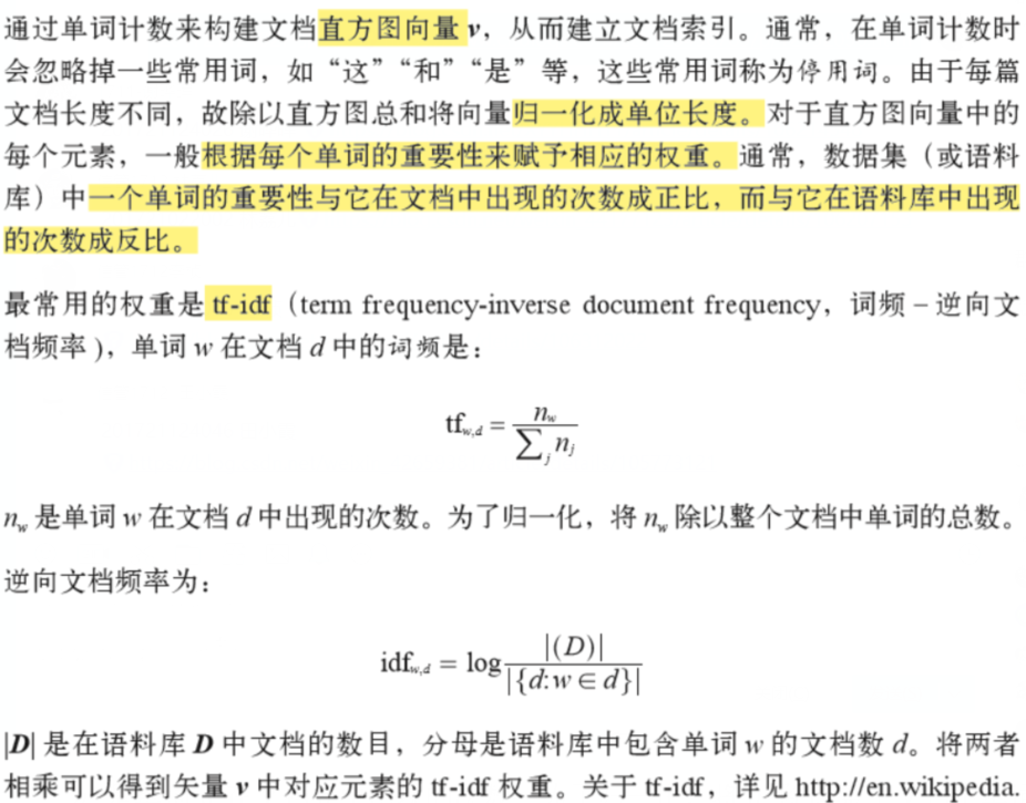
1.3TF—IDF

 

 

 

 

• 二、SIFT特征提取

 

由于图像中的词汇不像文本文档那样是现成的单词，所以我们首先要从图像中提取出相互独立的视觉词汇。然后为创建视觉单词词汇，第一步要做的就是提取特征描述子。
SIFT算法是提取图像中局部不变特征的应用最广的算法，所以我们可以采用SIFT算法才进行特征提取。
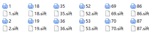
将每幅图像提取出的描述子保存在一个文件中，构建视觉词典。

# -*- coding: utf-8 -*-

import pickle

from PCV.imagesearch import vocabulary

from PCV.tools.imtools import get_imlist

import sift

# 获取图像列表

imlist = get_imlist('D:/Python/ComputerView/test1/first1000/')

nbr_images = len(imlist)

# 获取特征列表

featlist = [imlist[i][:-3] + 'sift' for i in range(nbr_images)]

# 提取文件夹下图像的sift特征

for i in range(nbr_images):
    sift.process_image(imlist[i], featlist[i])

# 生成词汇

voc = vocabulary.Vocabulary('ukbenchtest')

voc.train(featlist, 100, 10)

# 保存词汇

# saving vocabulary

with open('D:/Python/ComputerView/test1/first1000/vocabulary.pkl', 'wb') as f:

    pickle.dump(voc, f)

print('vocabulary is:', voc.name, voc.nbr_words)

 

 

• 三、视觉词典（visual vocabulary）

 

# -*- coding: utf-8 -*-
import pickle
from PCV.imagesearch import vocabulary
from PCV.tools.imtools import get_imlist
from PCV.localdescriptors import sift
 
#获取图像列表
imlist = get_imlist('first1000/')
nbr_images = len(imlist)
#获取特征列表
featlist = [imlist[i][:-3]+'sift' for i in range(nbr_images)]
 
#提取文件夹下图像的sift特征
for i in range(nbr_images):
    sift.process_image(imlist[i], featlist[i])
 
#生成词汇
voc = vocabulary.Vocabulary('ukbenchtest')
voc.train(featlist, 1000, 10)
#保存词汇
# saving vocabulary
with open('first1000/vocabulary.pkl', 'wb') as f:
    pickle.dump(voc, f)
print 'vocabulary is:', voc.name, voc.nbr_words

 

 

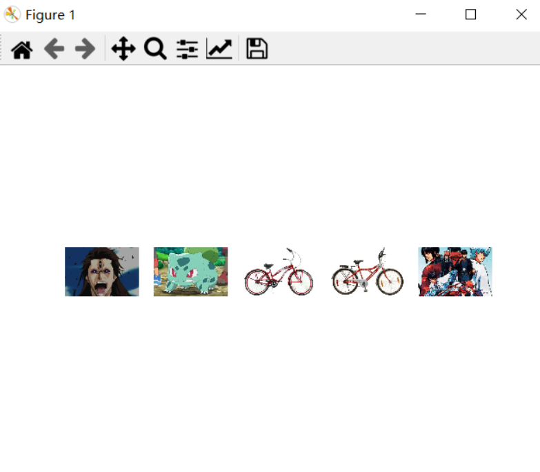
• 四、匹配 

# -*- coding: utf-8 -*-
import pickle
from PCV.localdescriptors import sift
from PCV.imagesearch import imagesearch
from PCV.geometry import homography
from PCV.tools.imtools import get_imlist

# load image list and vocabulary
#载入图像列表
imlist = get_imlist('D:/Study/untitled1/shiyan/')
nbr_images = len(imlist)
#载入特征列表
featlist = [imlist[i][:-3]+'sift' for i in range(nbr_images)]

#载入词汇
with open(r'D:/Study/untitled1/shiyan/vocabulary.pkl', 'rb') as f:
    voc = pickle.load(f)

src = imagesearch.Searcher('testImaAdd3.db',voc)

# index of query image and number of results to return
#查询图像索引和查询返回的图像数
q_ind = 6
nbr_results = 5

# regular query
# 常规查询(按欧式距离对结果排序)
res_reg = [w[1] for w in src.query(imlist[q_ind])[:nbr_results]]
print ('top matches (regular):', res_reg)

# load image features for query image
#载入查询图像特征
q_locs,q_descr = sift.read_features_from_file(featlist[q_ind])
fp = homography.make_homog(q_locs[:,:2].T)

# RANSAC model for homography fitting
#用单应性进行拟合建立RANSAC模型
model = homography.RansacModel()
rank = {}

# load image features for result
#载入候选图像的特征
for ndx in res_reg[1:]:
    locs,descr = sift.read_features_from_file(featlist[ndx])  # because 'ndx' is a rowid of the DB that starts at 1
    # get matches
    matches = sift.match(q_descr,descr)
    ind = matches.nonzero()[0]
    ind2 = matches[ind]
    tp = homography.make_homog(locs[:,:2].T)
    # compute homography, count inliers. if not enough matches return empty list
    try:
        H,inliers = homography.H_from_ransac(fp[:,ind],tp[:,ind2],model,match_theshold=4)
    except:
        inliers = []
    # store inlier count
    rank[ndx] = len(inliers)

# sort dictionary to get the most inliers first
sorted_rank = sorted(rank.items(), key=lambda t: t[1], reverse=True)
res_geom = [res_reg[0]]+[s[0] for s in sorted_rank]
print ('top matches (homography):', res_geom)

# 显示查询结果
imagesearch.plot_results(src,res_reg[:8]) #常规查询
imagesearch.plot_results(src,res_geom[:8]) #重排后的结果

 

• 五、TF-IDF解算

 

#train()函数
    def train(self,featurefiles,k=100,subsampling=10):
        """ Train a vocabulary from features in files listed 
            in featurefiles using k-means with k number of words. 
            Subsampling of training data can be used for speedup. """
        
        nbr_images = len(featurefiles)
        # read the features from file
        descr = []
        descr.append(sift.read_features_from_file(featurefiles[0])[1])
        descriptors = descr[0] #stack all features for k-means
        for i in arange(1,nbr_images):
            descr.append(sift.read_features_from_file(featurefiles[i])[1])
            descriptors = vstack((descriptors,descr[i]))
            
        # k-means: last number determines number of runs
        self.voc,distortion = kmeans(descriptors[::subsampling,:],k,1)#K-means算法
        self.nbr_words = self.voc.shape[0]
        
        # go through all training images and project on vocabulary
        imwords = zeros((nbr_images,self.nbr_words))
        for i in range( nbr_images ):
            imwords[i] = self.project(descr[i])
        
        nbr_occurences = sum( (imwords > 0)*1 ,axis=0)
        
        self.idf = log( (1.0*nbr_images) / (1.0*nbr_occurences+1) )
        self.trainingdata = featurefiles

 

 

 

• 六、检索

• # -*- coding: utf-8 -*-
  import pickle
  from PCV.imagesearch import imagesearch
  from PCV.localdescriptors import sift
  from sqlite3 import dbapi2 as sqlite
  from PCV.tools.imtools import get_imlist
   
  #获取图像列表
  imlist = get_imlist('first1000/')
  nbr_images = len(imlist)
  #获取特征列表
  featlist = [imlist[i][:-3]+'sift' for i in range(nbr_images)]
   
  # load vocabulary
  #载入词汇
  with open('first1000/vocabulary.pkl', 'rb') as f:
      voc = pickle.load(f)
  #创建索引
  indx = imagesearch.Indexer('testImaAdd.db',voc)
  indx.create_tables()
  # go through all images, project features on vocabulary and insert
  #遍历所有的图像，并将它们的特征投影到词汇上
  for i in range(nbr_images)[:1000]:
      locs,descr = sift.read_features_from_file(featlist[i])
      indx.add_to_index(imlist[i],descr)
  # commit to database
  #提交到数据库
  indx.db_commit()
   
  con = sqlite.connect('testImaAdd.db')
  print con.execute('select count (filename) from imlist').fetchone()
  print con.execute('select * from imlist').fetchone()

  

• 常规查询结果

 

 

 

• 重排后查询结果

• 七、总结

1.不选去有文字的图片尽心检索应该会使结果更好一些。数据集中也最好不要出现文字图片，数据集是表情包，所以难免会有文字在其中。

BOF算法还有一个明显的不足，就是它完全没有考虑到特征之间的位置关系，而位置信息对于人理解图片来说，作用是很明显的。 而且在提取特征时不需要相关的 label 进行学习，因此是一种弱监督的学习方法。

 

 

2.影响测试正确率的因素如下：

 

字典大小的选择是问题，字典过大，单词缺乏一般性，对噪声敏感，计算量大，关键是图象投影后的维数高；字典太小，单词区分性能差，对相似的目标特征无法表示。
使用k-means聚类，除了其K和初始聚类中心选择的问题外，对于海量数据，输入矩阵的巨大将使得内存溢出及效率低下。有方法是在海量图片中抽取部分训练集分类，使用朴素贝叶斯分类的方法对图库中其余图片进行自动分类。另外，由于图片爬虫在不断更新后台图像集，重新聚类的代价显而易见。
相似性测度函数用来将图象特征分类到单词本的对应单词上，其涉及线型核，塌方距离测度核，直方图交叉核等的选择。