

计算视觉——基础矩阵和极点极线
- 基础矩阵
在计算机视觉中,基础矩阵(Fundamental matrix)F是一个3×3的矩阵,表达了立体像对的像点之间的对应关系。在对极几何中,对于立体像对中的一对同名点,它们的齐次化图像坐标分别为p与 p',

F矩阵中蕴含了立体像对的两幅图像在拍摄时相互之间的空间几何关系(外参数)以及相机检校参数(内参数),包括旋转、位移、像主点坐标和焦距。因为F矩阵的秩为2,并且可以自由缩放(尺度化),所以只需7对同名点即可估算出F的值。
基础矩阵这一概念由Q. T. Luong在他那篇很有影响力的博士毕业论文中提出。
[1] Faugeras则是在1992年发表的著作
[2] 中以上面的关系式给出了F矩阵的定义。尽管Longuet-Higgins提出的本质矩阵也满足类似的关系式,但本质矩阵中并不蕴含相机检校参数。
本质矩阵与基础矩阵之间的关系可由下式表达:

其中K和K'分别为两个相机的内参数矩阵。
- 极点和极线
- 极点
- 极线
在数学中, 极线通常是一个适用于圆锥曲线的概念,如果圆锥曲线的切于A,B两点的切线相交于P点,那么P点称为直线AB关于该曲线的极点(pole),直线AB称为P点的极线(polar)。
- 极线的几何定义
上面定义仅适用于P点在此圆锥曲线外部的情况。实际上,在P点在圆锥曲线内部的时候同样可以定义极线,这时我们可以认为极线是过P点做此圆锥曲线两条虚切线切点的连线.特别的,如果这个圆锥曲线是一个圆,我们同样有圆的极线和极点的概念。
- 极线的几何性质
对于圆锥曲线,两个点的切线的交点的极线即这两点的连线。 [2] 此外,过不在圆锥曲线上任意一点做两条和此曲线相交的直线得出四个点,那么这四个点确定的四边形的对角线交点在该点的极线。我们也可以把这个性质作为圆锥曲线的极线的定义。 [3]
而当一个动点移动到曲线上,那么它的极线就退化为过这点的切线, 所以,极点和极线的思想实际上是曲线上点和过该点切线的思想的一般化。
- 求解图像之间的基础矩阵
1.归一化8点算法
基本矩阵是由下述方程定义
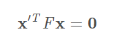
其中x相对于x′是两幅图像的任意一对匹配点。由于每一组点的匹配提供了计算FF系数的一个线性方程,当给定至少77个点(3×33×3的齐次矩阵减去一个尺度,以及一个秩为22的约束),方程就可以计算出未知的FF。
我们记点的坐标为x=(x,y,1)^T,x'=(x',y',1)^T,x=(x,y,1)^ T,x′=(x′,y′,1) ^T
则对应的方程为
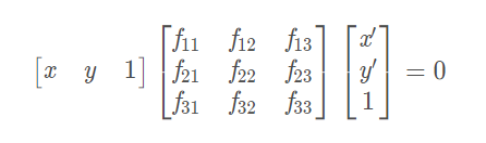
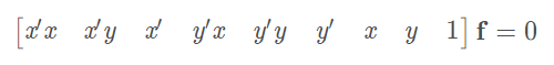
展开后有

把矩阵FFF写成列向量的形式,则有:
给定n组点的集合,我们有如下方程:
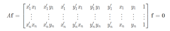
如果存在确定(非零)解,则系数矩阵A的秩最多是8。由于F是齐次矩阵,所以如果矩阵A的秩为8,则在差一个尺度因子的情况下解是唯一的。可以直接用线性算法解得。
最终解为

- 生成基础矩阵
from PIL import Image
from numpy import *
from pylab import *
import numpy as np

import PCV.geometry.camera as camera
import PCV.geometry.homography as homography
import PCV.geometry.sfm as sfm
import PCV.localdescriptors.sift as sift

im1 = array(Image.open('002.jpg'))
sift.process_image('002.jpg', 'im1.sift')

im2 = array(Image.open('001.jpg'))
sift.process_image('001.jpg', 'im2.sift')

l1, d1 = sift.read_features_from_file('im1.sift')
l2, d2 = sift.read_features_from_file('im2.sift')

matches = sift.match_twosided(d1, d2)

ndx = matches.nonzero()[0]
x1 = homography.make_homog(l1[ndx, :2].T)
ndx2 = [int(matches[i]) for i in ndx]
x2 = homography.make_homog(l2[ndx2, :2].T)

d1n = d1[ndx]
d2n = d2[ndx2]
x1n = x1.copy()
x2n = x2.copy()

figure(figsize=(16,16))
sift.plot_matches(im1, im2, l1, l2, matches, True)
show()

def F_from_ransac(x1, x2, model, maxiter=5000, match_threshold=1e-6):
    """ Robust estimation of a fundamental matrix F from point
    correspondences using RANSAC (ransac.py from
    http://www.scipy.org/Cookbook/RANSAC).

    input: x1, x2 (3*n arrays) points in hom. coordinates. """

    import PCV.tools.ransac as ransac
    data = np.vstack((x1, x2))
    d = 10 # 20 is the original
    F, ransac_data = ransac.ransac(data.T, model,
                                   8, maxiter, match_threshold, d, return_all=True)
    return F, ransac_data['inliers']

model = sfm.RansacModel()
F, inliers = F_from_ransac(x1n, x2n, model, maxiter=5000, match_threshold=1e-5)
print F

P1 = array([[1, 0, 0, 0], [0, 1, 0, 0], [0, 0, 1, 0]])
P2 = sfm.compute_P_from_fundamental(F)

X = sfm.triangulate(x1n[:, inliers], x2n[:, inliers], P1, P2)


cam1 = camera.Camera(P1)
cam2 = camera.Camera(P2)
x1p = cam1.project(X)
x2p = cam2.project(X)

figure(figsize=(16, 16))
imj = sift.appendimages(im1, im2)
imj = vstack((imj, imj))

imshow(imj)

cols1 = im1.shape[1]
rows1 = im1.shape[0]
for i in range(len(x1p[0])):
    if (0<= x1p[0][i]<cols1) and (0<= x2p[0][i]<cols1) and (0<=x1p[1][i]<rows1) and (0<=x2p[1][i]<rows1):
        plot([x1p[0][i], x2p[0][i]+cols1],[x1p[1][i], x2p[1][i]],'c')
axis('off')
show()

d1p = d1n[inliers]
d2p = d2n[inliers]

# Read features
im3 = array(Image.open('003.jpg'))
sift.process_image('003.jpg', 'im3.sift')
l3, d3 = sift.read_features_from_file('im3.sift')

matches13 = sift.match_twosided(d1p, d3)

ndx_13 = matches13.nonzero()[0]
x1_13 = homography.make_homog(x1p[:, ndx_13])
ndx2_13 = [int(matches13[i]) for i in ndx_13]
x3_13 = homography.make_homog(l3[ndx2_13, :2].T)

figure(figsize=(16, 16))
imj = sift.appendimages(im1, im3)
imj = vstack((imj, imj))

imshow(imj)

cols1 = im1.shape[1]
rows1 = im1.shape[0]
for i in range(len(x1_13[0])):
    if (0<= x1_13[0][i]<cols1) and (0<= x3_13[0][i]<cols1) and (0<=x1_13[1][i]<rows1) and (0<=x3_13[1][i]<rows1):
        plot([x1_13[0][i], x3_13[0][i]+cols1],[x1_13[1][i], x3_13[1][i]],'c')
axis('off')
show()

P3 = sfm.compute_P(x3_13, X[:, ndx_13])

print P1
print P2
print P3
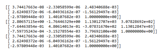
基础矩阵
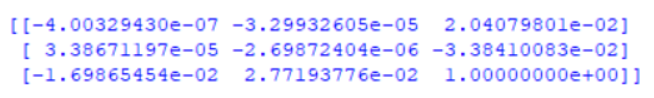
p1,p2,p3相机矩阵
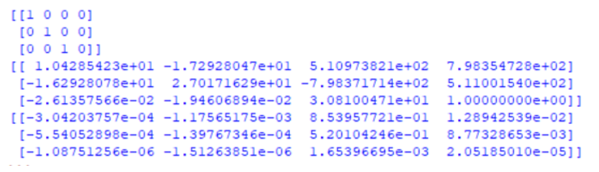

通过修改如图所示参数,可以修改为7点法或10点法
- 极线代码
import numpy as np
import cv2 as cv
from matplotlib import pyplot as plt


def drawlines(img1, img2, lines, pts1, pts2):
    ''' img1 - image on which we draw the epilines for the points in img2
        lines - corresponding epilines '''
    r, c = img1.shape
    img1 = cv.cvtColor(img1, cv.COLOR_GRAY2BGR)
    img2 = cv.cvtColor(img2, cv.COLOR_GRAY2BGR)
    for r, pt1, pt2 in zip(lines, pts1, pts2):
        color = tuple(np.random.randint(0, 255, 3).tolist())
        x0, y0 = map(int, [0, -r[2] / r[1]])
        x1, y1 = map(int, [c, -(r[2] + r[0] * c) / r[1]])
        img1 = cv.line(img1, (x0, y0), (x1, y1), color, 1)
        img1 = cv.circle(img1, tuple(pt1), 5, color, -1)
        img2 = cv.circle(img2, tuple(pt2), 5, color, -1)
    return img1, img2


img1 = cv.imread('D:/Study/untitled1/333/5.jpg', 0)  # queryimage # left image
img2 = cv.imread('D:/Study/untitled1/333/6.jpg', 0)  # trainimage # right image
sift = cv.xfeatures2d.SIFT_create()
# find the keypoints and descriptors with SIFT
kp1, des1 = sift.detectAndCompute(img1, None)
kp2, des2 = sift.detectAndCompute(img2, None)
# FLANN parameters
FLANN_INDEX_KDTREE = 1
index_params = dict(algorithm=FLANN_INDEX_KDTREE, trees=5)
search_params = dict(checks=50)
flann = cv.FlannBasedMatcher(index_params, search_params)
matches = flann.knnMatch(des1, des2, k=2)
good = []
pts1 = []
pts2 = []
# ratio test as per Lowe's paper
for i, (m, n) in enumerate(matches):
    if m.distance < 0.8 * n.distance:
        good.append(m)
        pts2.append(kp2[m.trainIdx].pt)
        pts1.append(kp1[m.queryIdx].pt)

pts1 = np.int32(pts1)
pts2 = np.int32(pts2)
F, mask = cv.findFundamentalMat(pts1, pts2, cv.FM_LMEDS)
# We select only inlier points
pts1 = pts1[mask.ravel() == 1]
pts2 = pts2[mask.ravel() == 1]

# Find epilines corresponding to points in right image (second image) and
# drawing its lines on left image
lines1 = cv.computeCorrespondEpilines(pts2.reshape(-1, 1, 2), 2, F)
lines1 = lines1.reshape(-1, 3)
img5, img6 = drawlines(img1, img2, lines1, pts1, pts2)
# Find epilines corresponding to points in left image (first image) and
# drawing its lines on right image
lines2 = cv.computeCorrespondEpilines(pts1.reshape(-1, 1, 2), 1, F)
lines2 = lines2.reshape(-1, 3)
img3, img4 = drawlines(img2, img1, lines2, pts2, pts1)
plt.subplot(121), plt.imshow(img5)
plt.subplot(122), plt.imshow(img3)
plt.show()
- 实验结果及分析
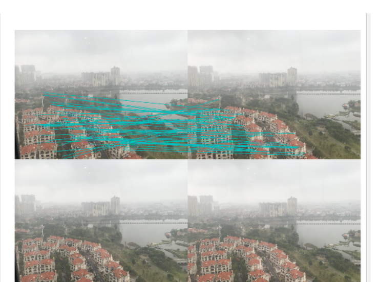
sift特征匹配:
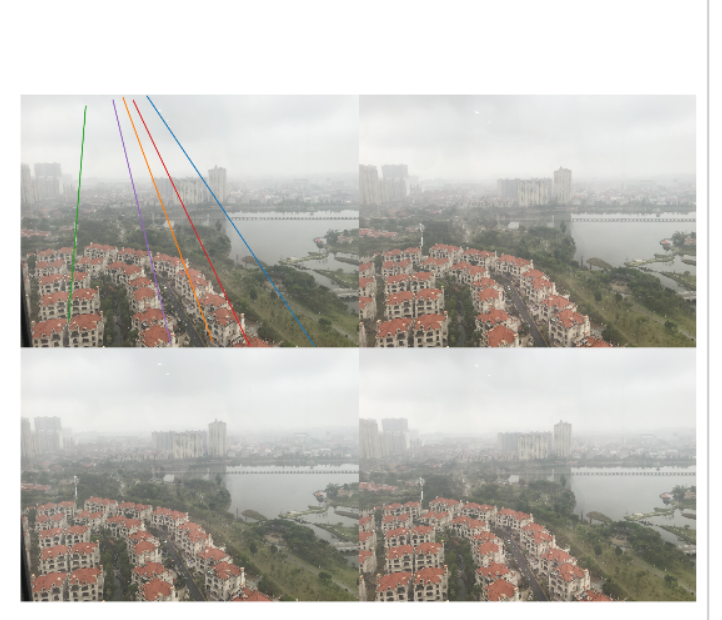
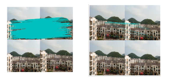
极点极线

- 实验总结
1. 在计算基础矩阵时多次报错或失败,原因经了解主要是图像压缩之后会丢失很多匹配特征点,因此在计算基础矩阵是一定要控制好图像压缩大小
2. 由于两幅图像在匹配的时候有不少错误的匹配,所以计算的基本矩阵有较大的误差。左右视图中都可以发现很多的点在对极线附近但并没有完全落在对极线上。我们可以观察到左右视图的对极线都响应地汇聚到一点,那点就是极点。这一对匹配中极点都落在图像内,当然也有些情况对极线会落在图像外
3. 8点算法是计算基本矩阵的最简单的方法。为了提高解的稳定性和精度,往往会对输入点集的坐标先进行归一化处理。
4. 计算 基础矩阵的前提是要先得到其sift特征匹配结果,通过sift特征匹配结果得到F基础矩阵,因此要确保sift寻找出更多的特征匹配点。

 浙公网安备 33010602011771号