深度学习（十二）——神经网络：搭建小实战和Sequential的使用

一、torch.nn.Sequential代码栗子

官方文档：Sequential — PyTorch 2.0 documentation

# Using Sequential to create a small model. When `model` is run,
# input will first be passed to `Conv2d(1,20,5)`. The output of
# `Conv2d(1,20,5)` will be used as the input to the first
# `ReLU`; the output of the first `ReLU` will become the input
# for `Conv2d(20,64,5)`. Finally, the output of
# `Conv2d(20,64,5)` will be used as input to the second `ReLU`
model = nn.Sequential(
          nn.Conv2d(1,20,5),
          nn.ReLU(),
          nn.Conv2d(20,64,5),
          nn.ReLU()
        )

• 在第一个变量名model中，依次执行nn.Convd2d(1,20,5)、nn.ReLU()、nn.Conv2d(20,64,5)、nn.ReLU()四个函数。这样写起来的好处是使代码更简洁。

• 由此可见，函数\(Sequential\)的主要作用为依次执行括号内的函数

二、神经网络搭建实战

采用\(CIFAR10\)中的数据，并对其进行简单的分类。以下图为例：

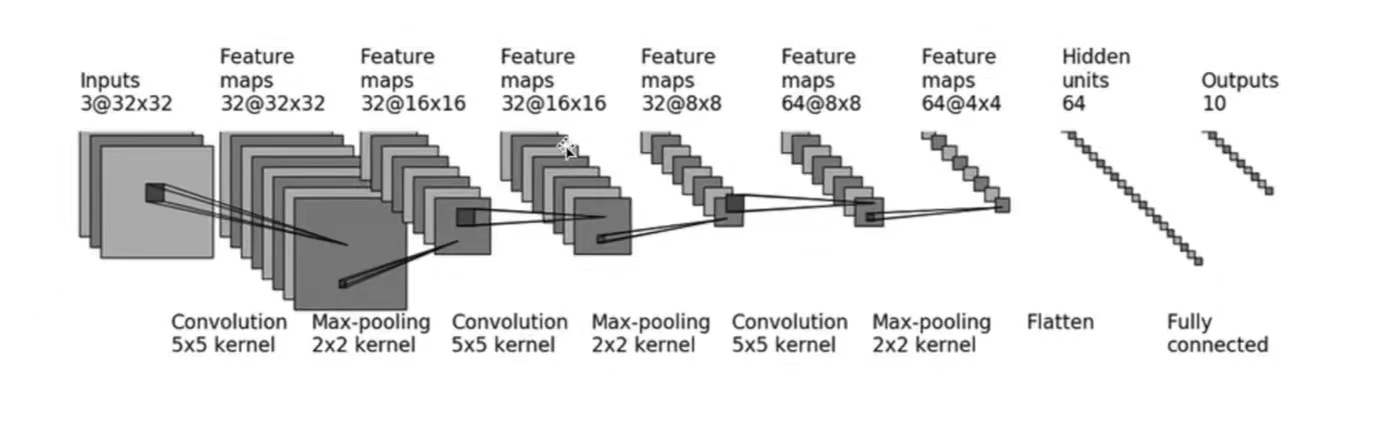
• 输入：3通道，32×32 → 经过一个5×5的卷积 → 变成32通道，32×32的图像 → 经过2×2的最大池化 → 变成32通道，16×16的图像.... → ... → 变成64通道，4×4的图像 → 把图像展平（Flatten）→ 变成64通道，1×1024 （64×4×4） 的图像 → 通过两个线性层，最后\(out\_feature=10\) → 得到最终图像

以上，就是CIFAR10模型的结构。本节的代码也基于CIFAR10 model的结构构建。

1. 神经网络中的参数设计及计算

（1）卷积层的参数设计（以第一个卷积层conv1为例）

• 输入图像为3通道，输出图像为32通道，故：\(in\_channels=3\)；\(out\_channels=32\)

• 卷积核尺寸为\(5×5\)

• 图像经过卷积层conv1前后的尺寸均为32×32，根据公式：

  \[H_{out}​=⌊\frac{H_{in}​+2×padding[0]−dilation[0]×(kernel\_size[0]−1)−1​}{stride[0]}+1⌋ \]
  \[W_{out}​=⌊\frac{W_{in}​+2×padding[1]−dilation[1]×(kernel\_size[1]−1)−1​}{stride[1]}+1⌋ \]

  可得：

  \[H_{out}​=⌊\frac{32​+2×padding[0]−1×(5−1)−1​}{stride[0]}+1⌋=32 \]
  \[W_{out}​=⌊\frac{32​+2×padding[1]−1×(5−1)−1​}{stride[1]}+1⌋=32 \]

  即：

  \[\frac{27+2×padding[0]​}{stride[0]}=31 \]
  \[\frac{27+2×padding[1]​}{stride[1]}=31 \]

  若\(stride[0]\)或\(stride[1]\)设置为2，那么上面的\(padding\)也会随之扩展为一个很大的数，这很不合理。所以这里设置：\(stride[0]=stride[1]=1\)，由此可得：\(padding[0]=padding[1]=2\)

其余卷积层的参数设计及计算方法均同上。

（2）最大池化操作的参数设计（以第一个池化操作maxpool1为例）

• 由图可得，\(kennel\_size=2\)

其余最大池化参数设计方法均同上。

（3）线性层的参数设计

• 通过三次卷积和最大池化操作后，图像尺寸变为64通道4×4。之后使用\(Flatten()\)函数将图像展成一列，此时图像尺寸变为：1×(64×4×4)，即\(1×1024\)

• 因此，之后通过第一个线性层，\(in\_features=1024\)，\(out\_features=64\)

• 通过第二个线性层，\(in\_features=64\)，\(out\_features=10\)

2. 构建神经网络实战

import torch
from torch import nn
from torch.nn import Conv2d, MaxPool2d, Flatten, Linear

class Demo(nn.Module):
    def __init__(self):
        super(Demo,self).__init__()

        # 搭建第一个卷积层:in_channels=3，out_channels=32，卷积核尺寸为5×5,通过计算得出：padding=2;stride默认情况下为1，不用设置
        self.conv1=Conv2d(3,32,5,padding=2)

        # 第一个最大池化操作,kennel_size=2
        self.maxpool1=MaxPool2d(2)

        # 第二个卷积层及最大池化操作
        self.conv2=Conv2d(32,32,5,padding=2)
        self.maxpool2=MaxPool2d(2)

        # 第三个卷积层及最大池化操作
        self.conv3=Conv2d(32,64,5,padding=2)
        self.maxpool3=MaxPool2d(2)

        # 展开图像
        self.flatten=Flatten()

        # 线性层参数设计
        self.linear1=Linear(1024,64)
        self.linear2=Linear(64,10)

        # 如果是预测概率，那么取输出结果的最大值（它代表了最大概率）

    def forward(self,x):
        x = self.conv1(x)
        x = self.maxpool1(x)
        x = self.conv2(x)
        x = self.maxpool2(x)
        x = self.conv3(x)
        x = self.maxpool3(x)
        x = self.flatten(x)
        x = self.linear1(x)   #如果线性层的1024和64不会计算，可以在self.flatten之后print(x.shape)查看尺寸，以此设定linear的参数
        x = self.linear2(x)
        return x

demo=Demo()
print(demo)
"""
[Run]
Demo(
  (conv1): Conv2d(3, 32, kernel_size=(5, 5), stride=(1, 1), padding=(2, 2))
  (maxpool1): MaxPool2d(kernel_size=2, stride=2, padding=0, dilation=1, ceil_mode=False)
  (conv2): Conv2d(32, 32, kernel_size=(5, 5), stride=(1, 1), padding=(2, 2))
  (maxpool2): MaxPool2d(kernel_size=2, stride=2, padding=0, dilation=1, ceil_mode=False)
  (conv3): Conv2d(32, 64, kernel_size=(5, 5), stride=(1, 1), padding=(2, 2))
  (maxpool3): MaxPool2d(kernel_size=2, stride=2, padding=0, dilation=1, ceil_mode=False)
  (flatten): Flatten(start_dim=1, end_dim=-1)
  (linear1): Linear(in_features=1024, out_features=64, bias=True)
  (linear2): Linear(in_features=64, out_features=10, bias=True)
)

可以看出，网络还是有模有样的
"""

#构建输入，测试神经网络
input=torch.ones((64,3,32,32))  #构建图像，batch_size=64,3通道,32×32
output=demo(input)
print(output.shape)  #[Run] torch.Size([64, 10])

这里的\(forward\)函数写的有点烦，这时候\(Sequential\)函数的优越就体现出来了（墨镜黄豆）。下面是\(class\) \(Demo\)优化后的代码：

class Demo(nn.Module):
    def __init__(self):
        super(Demo,self).__init__()

        self.model1=Sequential(
            Conv2d(3,32,5,padding=2),
            MaxPool2d(2),
            Conv2d(32, 32, 5, padding=2),
            MaxPool2d(2),
            Conv2d(32, 64, 5, padding=2),
            MaxPool2d(2),
            Flatten(),
            Linear(1024, 64),
            Linear(64, 10)
        )

    def forward(self,x):
        x=self.model1(x)
        return x

极简主义者看过后表示很满意ε٩(๑> ₃ <)۶з

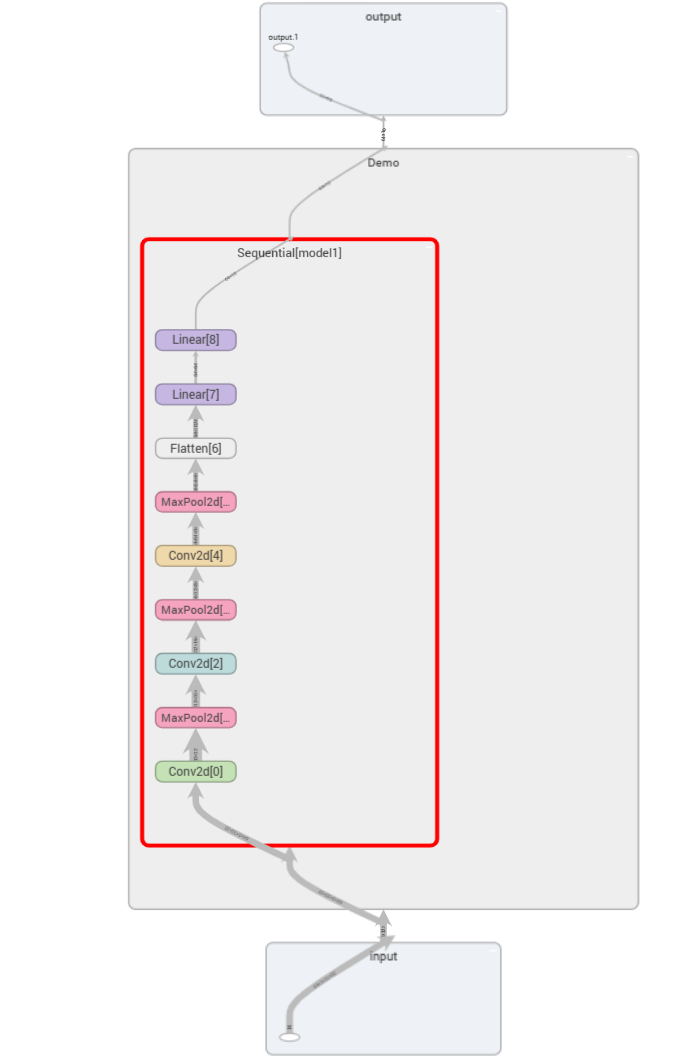
3. 可视化神经网络

from torch.utils.tensorboard import SummaryWriter
writer=SummaryWriter("logs_seq")
writer.add_graph(demo,input)
writer.close()

这样就可以清晰地看到神经网络的相关参数啦