《机器学习》周志华 习题答案9.4

原题采用Kmeans方法对西瓜数据集进行聚类。我花了一些时间居然没找到西瓜数据集4.0在哪里，于是直接采用sklearn给的例子来分析一遍，更能说明Kmeans的效果。

#!/usr/bin/python
# -*- coding:utf-8 -*-
import numpy as np
import matplotlib.pyplot as plt

from sklearn.ensemble import BaggingClassifier
from sklearn.tree import DecisionTreeClassifier

file1 = open('c:\quant\watermelon.csv','r')
data = [line.strip('\n').split(',') for line in file1]
data = np.array(data)
#X = [[float(raw[-7]),float(raw[-6]),float(raw[-5]),float(raw[-4]),float(raw[-3]), float(raw[-2])] for raw in data[1:,1:-1]]

X = [[float(raw[-3]), float(raw[-2])] for raw in data[1:]]
y = [1 if raw[-1]=='1' else 0 for raw in data[1:]]
X = np.array(X)
y = np.array(y)

print(__doc__)

from time import time
import numpy as np
import matplotlib.pyplot as plt

from sklearn import metrics
from sklearn.cluster import KMeans
from sklearn.datasets import load_digits
from sklearn.decomposition import PCA
from sklearn.preprocessing import scale

np.random.seed(42)

digits = load_digits()
data = scale(digits.data)
n_samples, n_features = data.shape
n_digits = len(np.unique(digits.target))
labels = digits.target

sample_size = 300

print("n_digits: %d, \t n_samples %d, \t n_features %d"
      % (n_digits, n_samples, n_features))
#一共十个不同的类

print(79 * '_')
print('% 9s' % 'init'
      '    time  inertia    homo   compl  v-meas     ARI AMI  silhouette')


def bench_k_means(estimator, name, data):
    t0 = time()
    estimator.fit(data)
    print('% 9s   %.2fs    %i   %.3f   %.3f   %.3f   %.3f   %.3f    %.3f'
          % (name, (time() - t0), estimator.inertia_,
             metrics.homogeneity_score(labels, estimator.labels_),
             metrics.completeness_score(labels, estimator.labels_),
             metrics.v_measure_score(labels, estimator.labels_),
             metrics.adjusted_rand_score(labels, estimator.labels_),
             metrics.adjusted_mutual_info_score(labels,  estimator.labels_),
             metrics.silhouette_score(data, estimator.labels_,
                                      metric='euclidean',
                                      sample_size=sample_size)))

#Homogeneity 和 completeness 表示簇的均一性和完整性。V值是他们的调和平均，值越大，说明效果越好。

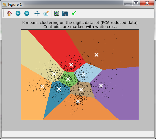
bench_k_means(KMeans(init='k-means++', n_clusters=n_digits, n_init=10),
              name="k-means++", data=data)

bench_k_means(KMeans(init='random', n_clusters=n_digits, n_init=10),
              name="random", data=data)

# in this case the seeding of the centers is deterministic, hence we run the
# kmeans algorithm only once with n_init=1
pca = PCA(n_components=n_digits).fit(data)
bench_k_means(KMeans(init=pca.components_, n_clusters=n_digits, n_init=1),
              name="PCA-based",
              data=data)
print(79 * '_')

###############################################################################
# Visualize the results on PCA-reduced data

reduced_data = PCA(n_components=2).fit_transform(data)
kmeans = KMeans(init='k-means++', n_clusters=n_digits, n_init=10)
kmeans.fit(reduced_data)

# Step size of the mesh. Decrease to increase the quality of the VQ.
h = .02     # point in the mesh [x_min, m_max]x[y_min, y_max].

# Plot the decision boundary. For that, we will assign a color to each
x_min, x_max = reduced_data[:, 0].min() - 1, reduced_data[:, 0].max() + 1
y_min, y_max = reduced_data[:, 1].min() - 1, reduced_data[:, 1].max() + 1
xx, yy = np.meshgrid(np.arange(x_min, x_max, h), np.arange(y_min, y_max, h))

# Obtain labels for each point in mesh. Use last trained model.
Z = kmeans.predict(np.c_[xx.ravel(), yy.ravel()])

# Put the result into a color plot
Z = Z.reshape(xx.shape)
plt.figure(1)
plt.clf()
plt.imshow(Z, interpolation='nearest',
           extent=(xx.min(), xx.max(), yy.min(), yy.max()),
           cmap=plt.cm.Paired,
           aspect='auto', origin='lower')

plt.plot(reduced_data[:, 0], reduced_data[:, 1], 'k.', markersize=2)
# Plot the centroids as a white X
centroids = kmeans.cluster_centers_
plt.scatter(centroids[:, 0], centroids[:, 1],
            marker='x', s=169, linewidths=3,
            color='w', zorder=10)
plt.title('K-means clustering on the digits dataset (PCA-reduced data)\n'
          'Centroids are marked with white cross')
plt.xlim(x_min, x_max)
plt.ylim(y_min, y_max)
plt.xticks(())
plt.yticks(())
plt.show()

运行文本结果：

n_digits: 10,      n_samples 1797,      n_features 64
_______________________________________________________________________________
init    time  inertia    homo   compl  v-meas     ARI AMI  silhouette
k-means++   0.21s    69432   0.602   0.650   0.625   0.465   0.598    0.146
   random   0.20s    69694   0.669   0.710   0.689   0.553   0.666    0.147
PCA-based   0.02s    71820   0.673   0.715   0.693   0.567   0.670    0.150

我们可以看到降维处理后运行时间缩短，而且V值还略高于以上两种方法。

图片结果：