python_数据分析与挖掘实战_客户流失预测

#7-1 数据探索
# 对数据进行基本的探索
#返回缺失值个数以及最大、最小值
# encoding:utf-8
import pandas as pd
datafile = './data/air_data.csv' # 航空原始数据，第一行为属性标签
resultfile = './data/aexplore.csv' # 数据探索结果表

data = pd.read_csv(datafile, encoding = 'utf-8')
# 包括对数据的基本描述，percentiles参数是指定计算多少的分位数表（如1/4分位数、中位数等）
explore = data.describe(percentiles = [], include = 'all').T
# describe()函数自动计算非空值数，需要手动计算空值
explore['null'] = len(data)-explore['count']

explore = explore[['null','max','min']]
explore.columns = [u'空值数', u'最大值', u'最小值'] #表头重命名
'''
这里只选取部分探索结果。
describe()函数自动计算的字段有count(非空值数)、unique(唯一指数)、top（频数最高者）、
freq（最高频数）、mean（平均值）、std（方差）、min（最小值）、50%（中位数）、max（最大值）
'''
explore.to_csv(resultfile)

# 7-2 探索客户的基本信息分布情况
# 客户信息类别
# 提取会员入会年份
from datetime import datetime
import matplotlib.pyplot as plt

ffp = data['FFP_DATE'].apply(lambda x:datetime.strptime(x,'%Y/%m/%d'))
ffp_year = ffp.map(lambda x : x.year)
# 绘制各年份会员入会人数直方图
fig = plt.figure(figsize=(8,5)) # 设置画布大小
plt.rcParams['font.sans-serif'] = ['SimHei'] #用来正常显示中文标签
plt.rcParams['axes.unicode_minus'] = False #用来显示负号
plt.hist(ffp_year, bins = 'auto', color='#0504aa')
plt.xlabel('年份')
plt.ylabel('入会人数')
plt.title('各年份会员入会人数 学号3142')
plt.show()
plt.close

# 提取会员不同性别人数
male = pd.value_counts(data['GENDER'])['男']
female = pd.value_counts(data['GENDER'])['女']
# 绘制会员性别比例饼图
fig = plt.figure(figsize=(7, 4)) # 设置画布大小
plt.pie([male,female],labels=['男','女'],colors=['lightskyblue','lightcoral'],autopct='%1.1f%%')
plt.title('会员性别比例 学号3142')
plt.show()
plt.close

#提取不同级别会员的人数
lv_four = pd.value_counts(data['FFP_TIER'])[4]
lv_five = pd.value_counts(data['FFP_TIER'])[5]
lv_six = pd.value_counts(data['FFP_TIER'])[6]

#绘制会员各级别人数条形图
fig = plt.figure(figsize=(8,5)) #设置画布大小
plt.bar(x=range(3),height=[lv_four,lv_five,lv_six], width=0.4, alpha=0.8, color='skyblue')
plt.xticks([index for index in range(3)],['4','5','6'])
plt.xlabel('会员等级')
plt.ylabel('会员人数')
plt.title('会员各级别人数 学号3142')
plt.show()
plt.close

# 提取会员年龄
age = data['AGE'].dropna()
age = age.astype('int64')
# 绘图会员年龄分布箱型图
fig = plt.figure(figsize=(5, 10))
plt.boxplot(age,
           patch_artist=True,
           labels = ['会员年龄'],   # 设置x轴标题
           boxprops = {'facecolor':'lightblue'}) # 设置填充颜色
plt.title('会员年龄分布箱型图 学号3142')
# 显示y坐标的底线
plt.grid(axis='y')
plt.show()
plt.close

 

 

 

# 7-3 探索客户乘机信息分布情况
lte = data['LAST_TO_END']
fc = data['FLIGHT_COUNT']
sks = data['SEG_KM_SUM']

#绘制最后乘机至结束时长箱型图
fig = plt.figure(figsize=(5,8))

plt.boxplot(lte,
            patch_artist=True,  
           labels = ['时长'], #设置x轴标题
           boxprops = {'facecolor':'lightblue'}) #设置填充颜色
plt.title('会员最后乘机至结束时长分布箱型图 学号3142')
#显示y坐标轴的底线
plt.grid(axis='y')
plt.show()
plt.close

#绘制客户飞行次数箱型图
fig = plt.figure(figsize=(5,8))
plt.boxplot(fc,
            patch_artist=True,  
           labels = ['飞行次数'], #设置x轴标题
           boxprops = {'facecolor':'lightblue'}) #设置填充颜色

plt.title('会员飞行次数分布箱型图 学号3142')
# 显示y坐标的底线
plt.grid(axis='y')
plt.show()
plt.close

# 绘制客户总飞行公里数箱型图
fig = plt.figure(figsize=(5,10))
plt.boxplot(sks,
           patch_artist=True,
           labels = ['总飞行公里数'],   # 设置x轴标题
           boxprops = {'facecolor':'lightblue'}) # 设置填充颜色
plt.title('客户总飞行公里数箱型图 学号3142')
# 显示y坐标的底线
plt.grid(axis='y')
plt.show()
plt.close

# 7-4 探索客户的积分信息分布情况
# 积分信息分类
# 提取会员积分兑换次数
ec = data['EXCHANGE_COUNT']

#绘制会员兑换积分次数直方图
fig = plt.figure(figsize=(8,5))
plt.hist(ec, bins=5, color='#0504aa')
plt.xlabel('兑换次数')
plt.ylabel('会员人数')
plt.title('会员兑换积分次数分布直方图 学号3142')
plt.show()
plt.close

# 提取会员总累计积分
ps = data['Points_Sum']
# 绘制会员总累计积分箱型图
fig = plt.figure(figsize=(5,8))
plt.boxplot(ps, 
            patch_artist=True,  
           labels = ['总累计积分'], #设置x轴标题
           boxprops = {'facecolor':'lightblue'}) #设置填充颜色
plt.title('客户总累计积分箱型图 学号3142')
#显示y坐标轴的底线
plt.grid(axis='y')
plt.show()
plt.close

# 7-5 相关系数矩阵与热力图
# 提取属性并合并为新数据集
data_corr = data[['FFP_TIER', 'FLIGHT_COUNT', 'LAST_TO_END', 'SEG_KM_SUM', 'EXCHANGE_COUNT', 'Points_Sum']]
age1 = data['AGE'].fillna(0)
data_corr['AGE'] = age1.astype('int64')
data_corr['ffp_year'] = ffp_year

#计算相关性矩阵
dt_corr = data_corr.corr(method='pearson')
print('相关性矩阵为：\n', dt_corr)

# 绘制热力图
import seaborn as sns
plt.subplots(figsize=(10, 10))
sns.heatmap(dt_corr, annot=True, vmax=1, square=True, cmap='Blues')
plt.title('学号3142')
plt.show()
plt.close

相关性矩阵为：
                 FFP_TIER  FLIGHT_COUNT  LAST_TO_END  SEG_KM_SUM  \
FFP_TIER        1.000000      0.582447    -0.206313    0.522350   
FLIGHT_COUNT    0.582447      1.000000    -0.404999    0.850411   
LAST_TO_END    -0.206313     -0.404999     1.000000   -0.369509   
SEG_KM_SUM      0.522350      0.850411    -0.369509    1.000000   
EXCHANGE_COUNT  0.342355      0.502501    -0.169717    0.507819   
Points_Sum      0.559249      0.747092    -0.292027    0.853014   
AGE             0.076245      0.075309    -0.027654    0.087285   
ffp_year       -0.116510     -0.188181     0.117913   -0.171508   

                EXCHANGE_COUNT  Points_Sum       AGE  ffp_year  
FFP_TIER              0.342355    0.559249  0.076245 -0.116510  
FLIGHT_COUNT          0.502501    0.747092  0.075309 -0.188181  
LAST_TO_END          -0.169717   -0.292027 -0.027654  0.117913  
SEG_KM_SUM            0.507819    0.853014  0.087285 -0.171508  
EXCHANGE_COUNT        1.000000    0.578581  0.032760 -0.216610  
Points_Sum            0.578581    1.000000  0.074887 -0.163431  
AGE                   0.032760    0.074887  1.000000 -0.242579  
ffp_year             -0.216610   -0.163431 -0.242579  1.000000  

 

#代码7-6 清洗空值与异常值
import numpy as np
import pandas as pd

datafile = "./data/air_data.csv"
cleanedfile = "./data/data_cleaned.csv"

#读取数据
airline_data = pd.read_csv(datafile,encoding = 'utf-8')
print('原始数据的形状为:',airline_data.shape)

#去除票价为空的记录
airline_notnull = airline_data.loc[airline_data['SUM_YR_1'].notnull() &
                                  airline_data['SUM_YR_2'].notnull(),:]
print('删除缺失记录后数据的形状为：',airline_notnull.shape)

# 只保留票价非零的，或者平均折扣率不为0且总飞行公里数大于0的记录
index1 = airline_notnull['SUM_YR_1'] != 0
index2 = airline_notnull['SUM_YR_2'] != 0
index3 = (airline_notnull['SEG_KM_SUM']>0) & (airline_notnull['avg_discount'] != 0)
index4 = airline_notnull['AGE'] >100 # 去除年龄大于100的记录
airline = airline_notnull[(index1 | index2) & index3 & ~index4]
print('数据清洗后数据的形状为：', airline.shape)

airline.to_csv(cleanedfile) # 保存清洗后的数据

原始数据的形状为: (62988, 44)
删除缺失记录后数据的形状为： (62299, 44)
数据清洗后数据的形状为： (62043, 44)

# 7-7 属性选择
import pandas as pd
import numpy as np

# 读取数据清洗后的数据
cleanedfile = "./data/data_cleaned.csv" # 数据清洗后保存的文件路径
airline = pd.read_csv(cleanedfile, encoding='utf-8')
# 选取需求属性
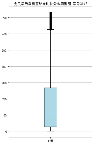
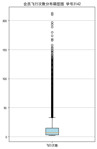
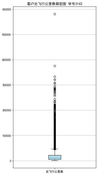
airline_selection = airline[['FFP_DATE', 'LOAD_TIME', 'LAST_TO_END', 'FLIGHT_COUNT', 'SEG_KM_SUM', 'avg_discount']]
print('筛选的属性前5行为：\n', airline_selection.head())

筛选的属性前5行为：
     FFP_DATE  LOAD_TIME  LAST_TO_END  FLIGHT_COUNT  SEG_KM_SUM  avg_discount
0  2006/11/2  2014/3/31            1           210      580717      0.961639
1  2007/2/19  2014/3/31            7           140      293678      1.252314
2   2007/2/1  2014/3/31           11           135      283712      1.254676
3  2008/8/22  2014/3/31           97            23      281336      1.090870
4  2009/4/10  2014/3/31            5           152      309928      0.970658

# 7-8 属性构造与数据标准化
# 构造属性L
L = pd.to_datetime(airline_selection['LOAD_TIME']) -  pd.to_datetime(airline_selection['FFP_DATE'])
L = L.astype('str').str.split().str[0]
L = L.astype('int')/30

# 合并属性
airline_features = pd.concat([L,airline_selection.iloc[:,2:]],axis=1)
print('构建的LRFMC属性前5行为：\n', airline_features.head())

# 数据标准化
from sklearn.preprocessing import StandardScaler
data = StandardScaler().fit_transform(airline_features)
np.savez('./data/airline_scale.npz', data)
print('标准化后LRFMC 5个属性为：\n', data[:5,:])

构建的LRFMC属性前5行为：
            0  LAST_TO_END  FLIGHT_COUNT  SEG_KM_SUM  avg_discount
0  90.200000            1           210      580717      0.961639
1  86.566667            7           140      293678      1.252314
2  87.166667           11           135      283712      1.254676
3  68.233333           97            23      281336      1.090870
4  60.533333            5           152      309928      0.970658
标准化后LRFMC 5个属性为：
 [[ 1.43579256 -0.94493902 14.03402401 26.76115699  1.29554188]
 [ 1.30723219 -0.91188564  9.07321595 13.12686436  2.86817777]
 [ 1.32846234 -0.88985006  8.71887252 12.65348144  2.88095186]
 [ 0.65853304 -0.41608504  0.78157962 12.54062193  1.99471546]
 [ 0.3860794  -0.92290343  9.92364019 13.89873597  1.34433641]]

#代码7-9 K-Meas聚类标准化后的数据
import pandas as pd
import numpy as np
from sklearn.cluster import KMeans #导入K-Mmeans算法

#读取标准化后的数据
airline_scale = np.load('./data/airline_scale.npz')['arr_0']
k = 5 #确定聚类中心数

#构建模型，随机种子设为123
kmeans_model = KMeans(n_clusters=k,random_state=123)
fit_kmeans = kmeans_model.fit(airline_scale) #模型训练

#查看聚类结果
kmeans_cc = kmeans_model.cluster_centers_ #聚类中心
print('各聚类中心为：\n',kmeans_cc)
kmeans_labels = kmeans_model.labels_ #样本的类别标签
print('各样本的类别标签为：\n',kmeans_labels)
r1 = pd.Series(kmeans_model.labels_).value_counts() #统计不同类别样本的数目
print('最终每个类别的数目为：\n',r1)
#输出聚类分群的结果
cluster_center = pd.DataFrame(kmeans_model.cluster_centers_,\
                             columns = ['ZL','ZR','ZF','ZM','ZC']) #将聚类中心放在数据中
cluster_center.index = pd.DataFrame(kmeans_model.labels_).\
                             drop_duplicates().iloc[:,0] #将样本类别作为数据框索引
print(cluster_center)

各聚类中心为：
 [[-0.70030628 -0.41502288 -0.16081841 -0.16053724 -0.25728596]
 [ 0.0444681  -0.00249102 -0.23046649 -0.23492871  2.17528742]
 [ 0.48370858 -0.79939042  2.48317171  2.42445742  0.30923962]
 [ 1.1608298  -0.37751261 -0.08668008 -0.09460809 -0.15678402]
 [-0.31319365  1.68685465 -0.57392007 -0.5367502  -0.17484815]]
各样本的类别标签为：
 [2 2 2 ... 0 4 4]
最终每个类别的数目为：
 0    24630
3    15733
4    12117
2     5337
1     4226
dtype: int64
         ZL        ZR        ZF        ZM        ZC
0                                                  
2 -0.700306 -0.415023 -0.160818 -0.160537 -0.257286
1  0.044468 -0.002491 -0.230466 -0.234929  2.175287
3  0.483709 -0.799390  2.483172  2.424457  0.309240
0  1.160830 -0.377513 -0.086680 -0.094608 -0.156784
4 -0.313194  1.686855 -0.573920 -0.536750 -0.174848

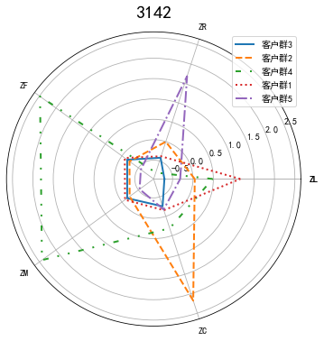
# 7-10 绘制客户分群雷达图
from sklearn.cluster import KMeans
airline_scale = np.load('./data/airline_scale.npz')['arr_0']
k = 5
kmeans_model = KMeans(n_clusters=k,  random_state=123)
fit_kmeans = kmeans_model.fit(airline_scale)
kmeans_cc = kmeans_model.cluster_centers_
kmeans_labels = kmeans_model.labels_
r1 = pd.Series(kmeans_model.labels_).value_counts()
cluster_center = pd.DataFrame(kmeans_model.cluster_centers_,columns=['ZL','ZR','ZF','ZM','ZC'])
cluster_center.index = pd.DataFrame(kmeans_model.labels_).drop_duplicates().iloc[:,0]
print(cluster_center)
labels = ['ZL','ZR','ZF','ZM','ZC']
# labels = labels.append('ZL')
legen = ['客户群' + str(i + 1) for i in cluster_center.index]
lstype = ['-','--',(0,(3,5,1,5,1,5)),':','-.']
kinds = list(cluster_center.iloc[:,0])


cluster_center = pd.concat([cluster_center,cluster_center[['ZL']]], axis=1)
centers = np.array(cluster_center.iloc[:,0:])

n = len(labels)
angle = np.linspace(0, 2*np.pi, n, endpoint=False)
# print([angle[0]])
angle = np.concatenate((angle, [angle[0]]))
labels = np.concatenate((labels, [labels[0]]))
fig = plt.figure(figsize=(8,6))
ax = fig.add_subplot(111,polar=True)
plt.rcParams['font.sans-serif'] = ['SimHei']
plt.rcParams['axes.unicode_minus'] = False

# print(cluster_center)
# print(centers)
# print(angle)

for i in range(len(kinds)):
    ax.plot(angle, centers[i], linestyle=lstype[i], linewidth=2, label=kinds[i])
# ax.plot(angle, centers, linestyle=lstype[i], linewidth=2, label=kinds[i])
ax.set_thetagrids(angle*180/np.pi,labels)
plt.title('3142',fontsize=20)
plt.legend(legen)
plt.show()
plt.close

import matplotlib.pyplot as plt
import pandas as pd
import numpy as np
import matplotlib.ticker as mtick
data = pd.read_csv('./data/WA_Fn-UseC_-Telco-Customer-Churn.csv')

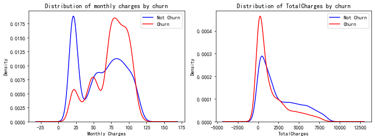
# #用密度图展现月消费、总消费与流失的关系
fig, ax = plt.subplots(1,2,figsize=(12,4))
data.MonthlyCharges[data['Churn'] == 'No'].plot(kind = 'kde',color ='blue',ax=ax[0])
data.MonthlyCharges[data['Churn'] == 'Yes'].plot(kind = 'kde',color ='red',ax=ax[0])
ax[0].legend(["Not Churn","Churn"],loc='upper right')
ax[0].set_ylabel('Density')
ax[0].set_xlabel('Monthly Charges')
ax[0].set_title('Distribution of monthly charges by churn')
ax[0].set_ylim(0)

#总消费需要转化数据类型，并把空值填充为0
data['TotalCharges'] = data['TotalCharges'].replace(" ", 0).astype('float')
data.TotalCharges[data['Churn'] == 'No'].plot(kind = 'kde',color ='blue',ax=ax[1])
data.TotalCharges[data['Churn'] == 'Yes'].plot(kind = 'kde',color ='red',ax=ax[1])
ax[1].legend(["Not Churn","Churn"],loc='upper right')
ax[1].set_ylabel('Density')
ax[1].set_xlabel('TotalCharges')
ax[1].set_title('Distribution of TotalCharges by churn')
ax[1].set_ylim(0)

# 对数据进行虚拟变量处理，也叫哑变量和离散特征编码，可用来表示分类变量、非数量因素可能产生的影响。
data_xy = data.drop(['customerID','gender','PhoneService','MultipleLines'],axis=1)
data_xy['Churn'].replace(to_replace='Yes', value=1, inplace=True)
data_xy['Churn'].replace(to_replace='No',  value=0, inplace=True)
data_dummies = pd.get_dummies(data_xy)

# 归一化数据
from sklearn.preprocessing import StandardScaler

standard = StandardScaler()
standard.fit(data_dummies[['tenure','MonthlyCharges','TotalCharges']])

data_dummies[['tenure','MonthlyCharges','TotalCharges']] = standard.transform(data_dummies[['tenure','MonthlyCharges','TotalCharges']])

#划分数据集
from sklearn.model_selection import train_test_split

X = data_dummies.drop('Churn', axis=1)
y = data_dummies['Churn']

X_train, X_test, y_train, y_test = train_test_split(X, y, test_size=0.3, random_state=101)

from sklearn.svm import SVC #支持向量机
from sklearn.linear_model import LogisticRegression #逻辑回归
from sklearn.naive_bayes import GaussianNB#朴素贝叶斯
from sklearn.tree import DecisionTreeClassifier#决策树分类器

from sklearn.metrics import recall_score,f1_score,precision_score, accuracy_score
Classifiers = [['SVM',SVC()],
              ['LogisticRegression',LogisticRegression()],
              ['GaussianNB',GaussianNB()],
              ['DecisionTreeClassifier',DecisionTreeClassifier()]]

Classify_results = []
names = []
prediction = []
for name ,classifier in Classifiers:
    classifier.fit(X_train,y_train)#训练这4个模型
    y_pred = classifier.predict(X_test)#预测这4个模型
    
    recall = recall_score(y_test,y_pred)#评估这四个模型的召回率
    precision = precision_score(y_test,y_pred)#评估这四个模型的精确率
    f1 = f1_score(y_test,y_pred)#评估这四个模型的f1分数
    acc = accuracy_score(y_test, y_pred)
    class_eva = pd.DataFrame([recall,precision,f1,acc])#将召回率、精确率和f1分数放在df中，方便接下来对比
    Classify_results.append(class_eva)
    name = pd.Series(name)
    names.append(name)
    y_pred = pd.DataFrame(y_pred)
    prediction.append(y_pred)
    
    
    pred = y_pred.values
    test = y_test.values
    i = 0
    sum = 0
    lost = 0
    norm = 0
    wlost = 0
    wnorm = 0
    for j in test:
        if(j == pred[i]):
            sum += 1
#             正确预测保留
            if( j == 0 ):
                norm += 1
#             正确预测流失
            elif( j == 1):
                lost += 1
        else:
#             错误预测保留
            if( j == 0 ):
                wnorm += 1
#             错误预测流失
            elif( j == 1):
                wlost += 1
        i = i + 1
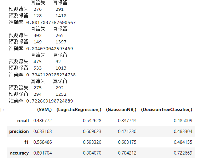
    print('\t真流失\t真保留')
    print('预测流失\t',lost,'\t',wlost)
    print('预测保留\t',wnorm,'\t',norm)
    print('准确率',sum/len(pred)) 

names = pd.DataFrame(names)
result = pd.concat(Classify_results,axis=1)
result.columns = names
result.index=[['recall','precision','f1','accuracy']]
result

 

 

	(SVM,)	(LogisticRegression,)	(GaussianNB,)	(DecisionTreeClassifier,)
recall	0.486772	0.532628	0.837743	0.485009
precision	0.683168	0.669623	0.471230	0.483304
f1	0.568486	0.593320	0.603175	0.484155
accuracy	0.801704	0.804070	0.704212	0.7226