第三周作业：卷积神经网络（Part1）

深度学习计算

层和块

层

通过实例化nn.Sequential来构建的模型，层的执行顺序是作为参数传递的。

import torch
from torch import nn
from torch.nn import functional as F
net = nn.Sequential(nn.Linear(20, 256), nn.ReLU(), nn.Linear(256, 10))
X = torch.rand(2, 20)
net(X)

块

#自定义块
class MLP(nn.Module):
    def __init__(self):
        super().__init__()
        self.hidden = nn.Linear(20, 256)
        self.out = nn.Linear(256, 10)

    def forward(self, X):
        return self.out(F.relu(self.hidden(X)))
net = MLP()
net(X)

#顺序块
class MySequential(nn.Module):
    def __init__(self, *args):
        super().__init__()
        for block in args:
            self._modules[block] = block

    def forward(self, X):
        for block in self._modules.values():
            X = block(X)
        return X

net = MySequential(nn.Linear(20, 256), nn.ReLU(), nn.Linear(256, 10))
net(X)

#在正向传播函数中执行代码
class FixedHiddenMLP(nn.Module):
    def __init__(self):
        super().__init__()
        self.rand_weight = torch.rand((20, 20), requires_grad=False)
        self.linear = nn.Linear(20, 20)

    def forward(self, X):
        X = self.linear(X)
        X = F.relu(torch.mm(X, self.rand_weight) + 1)
        X = self.linear(X)
        while X.abs().sum() > 1:
            X /= 2
        return X.sum()

net = FixedHiddenMLP()
net(X)

#混合搭配各种组合块的方法
class NestMLP(nn.Module):
    def __init__(self):
        super().__init__()
        self.net = nn.Sequential(nn.Linear(20, 64), nn.ReLU(),
                                 nn.Linear(64, 32), nn.ReLU())
        self.linear = nn.Linear(32, 16)

    def forward(self, X):
        return self.linear(self.net(X))

chimera = nn.Sequential(NestMLP(), nn.Linear(16, 20), FixedHiddenMLP())
chimera(X)

参数管理

#访问某层参数
import torch
from torch import nn

net = nn.Sequential(nn.Linear(4, 8), nn.ReLU(), nn.Linear(8, 1))
X = torch.rand(size=(2, 4))
net(X)
print(net[2].state_dict())

#一次性访问所有参数
for name, param in net.named_parameters():
  print(name)
print(*[(name, param.shape) for name, param in net[0].named_parameters()])
print(*[(name, param.shape) for name, param in net.named_parameters()])

#共享参数
shared = nn.Linear(8, 8)
net = nn.Sequential(nn.Linear(4, 8), nn.ReLU(), shared, nn.ReLU(), shared,
                    nn.ReLU(), nn.Linear(8, 1))
net(X)
print(net[2].weight.data[0] == net[4].weight.data[0])
net[2].weight.data[0, 0] = 100
print(net[2].weight.data[0] == net[4].weight.data[0])

#从嵌套块收集参数
def block1():
    return nn.Sequential(nn.Linear(4, 8), nn.ReLU(), nn.Linear(8, 4), nn.ReLU())

def block2():
    net = nn.Sequential()
    for i in range(4):
        net.add_module(f'block {i}', block1())
    return net

rgnet = nn.Sequential(block2(), nn.Linear(4, 1))
print(rgnet)
rgnet(X)

自定义层

#构造一个没有任何参数的自定义层
import torch
import torch.nn.functional as F
from torch import nn

class CenteredLayer(nn.Module):
    #def __init__(self):
        #super().__init__()

    def forward(self, X):
        return X - X.mean()

layer = CenteredLayer()
layer(torch.FloatTensor([1, 2, 3, 4, 5]))

#将层作为组件合并到构建更复杂的模型中
net = nn.Sequential(nn.Linear(8, 128), CenteredLayer())
#print(net.state_dict())
Y = net(torch.rand(4, 8))
class MyLinear(nn.Module):
    def __init__(self, in_units, units):
        super().__init__()
        self.weight = nn.Parameter(torch.randn(in_units, units))
        self.bias = nn.Parameter(torch.randn(units,))

    def forward(self, X):
        linear = torch.matmul(X, self.weight.data) + self.bias.data
        return F.relu(linear)

linear = MyLinear(5, 3)
linear.weight
#使用自定义层直接执行正向传播计算
linear(torch.rand(2, 5))
#使用自定义层构建模型
net = nn.Sequential(MyLinear(64, 8), MyLinear(8, 1))
net(torch.rand(2, 64))

存取参数

#读写文件
#加载和保存张量
import torch
from torch import nn
from torch.nn import functional as F

x = torch.arange(4)
torch.save(x, 'x-file')

x2 = torch.load('x-file')
x2

#存储一个张量列表，然后把它们读回内存
y = torch.zeros(4)
torch.save([x, y], 'x-files')
x2, y2 = torch.load('x-files')
(x2, y2)

#写入或读取从字符串映射到张量的字典
mydict = {'x': x, 'y': y}
print(mydict)
torch.save(mydict, 'mydict')
mydict2 = torch.load('mydict')
mydict2

#加载和保存模型参数
class MLP(nn.Module):
    def __init__(self):
        super().__init__()
        self.hidden = nn.Linear(20, 256)
        self.output = nn.Linear(256, 10)

    def forward(self, x):
        return self.output(F.relu(self.hidden(x)))

net = MLP()
X = torch.randn(size=(2, 20))
Y = net(X)

#将模型的参数存储为一个叫做“mlp.params”的文件
torch.save(net.state_dict(), 'mlp.params')

#实例化了原始多层感知机模型的一个备份。 直接读取文件中存储的参数
clone = MLP()
clone.load_state_dict(torch.load('mlp.params'))
clone.eval()
Y_clone = clone(X)
Y_clone == Y

GPU

#查询张量所在的设备
x = torch.tensor([1, 2, 3])
x.device
#存储在GPU上
X = torch.ones(2, 3, device=try_gpu())
X,X.device

#这两个函数允许我们在请求的GPU不存在的情况下运行代码
def try_gpu(i=0):  
    """如果存在，则返回gpu(i)，否则返回cpu()。"""
    if torch.cuda.device_count() >= i + 1:
        return torch.device(f'cuda:{i}')
    return torch.device('cpu')

def try_all_gpus():  
    """返回所有可用的GPU，如果没有GPU，则返回[cpu(),]。"""
    devices = [
        torch.device(f'cuda:{i}') for i in range(torch.cuda.device_count())]
    return devices if devices else [torch.device('cpu')]

try_gpu(), try_gpu(10), try_all_gpus()

#神经网络与GPU
net = nn.Sequential(nn.Linear(3, 1))
net = net.to(device=try_gpu())
net(X)

卷积神经网络

卷积层

平移不变性（translation invariance）：不管检测对象出现在图像中的哪个位置，神经网络的前面几层应该对相同的图像区域具有相似的反应，即为“平移不变性”。
局部性（locality）：神经网络的前面几层应该只探索输入图像中的局部区域，而不过度在意图像中相隔较远区域的关系，这就是“局部性”原则。最终，在后续神经网络，整个图像级别上可以集成这些局部特征用于预测。

import torch
from torch import nn
from d2l import torch as d2l
def corr2d(X,K):
  #计算二维互相关运算
  h,w = K.shape
  Y = torch.zeros((X.shape[0]-h+1,X.shape[1]-w+1))
  for i in range(Y.shape[0]):
    for j in range(Y.shape[1]):
      Y[i,j] = (X[i:i+h,j:j+w]*K).sum()
  return Y
X = torch.tensor([[0.0,1.0,2.0],[3.0,4.0,5.0],[6.0,7.0,8.0]])
K = torch.tensor([[0.0,1.0],[2.0,3.0]])
corr2d(X,K)

#实现二维卷积层
class Conv2D(nn.Module):
  def _init_(self,kernel_size):
    super()._init_()
    self.weight = nn.Parameter(torch.rand(kernel_size))
    self.bias = nn.Parameter(torch.zeros(1))
  def forward(self,x):
    return corr2d(x,self.weight)+self.bias

#卷积层的一个简单应用： 检测图像中不同颜色的边缘
X = torch.ones((6, 8))
X[:, 2:6] = 0
K = torch.tensor([[1.0,-1.0]])
Y = corr2d(X,K)

#学习由X生成Y的卷积核
conv2d = nn.Conv2d(1,1,kernel_size=(1,2),bias=False)
X = X.reshape((1,1,6,8))
Y = Y.reshape((1,1,6,7))
for i in range(10):
  Y_hat = conv2d(X)
  l = (Y_hat-Y)**2
  conv2d.zero_grad()
  l.sum().backward()
  conv2d.weight.data[:] -= 3e-2*conv2d.weight.grad
  if (i+1)%2 == 0:
    print(f'batch{i+1}, loss {l.sum():.3f}')
conv2d.weight.data.reshape((1,2))

#所学的卷积核的权重张量
conv2d.weight.data.reshape((1, 2))
tensor([[ 0.9905, -0.9963]])

填充和步幅

#Padding
def comp_conv2d(conv2d,X):
  X = X.reshape((1,1)+X.shape)
  #print(X.shape)
  Y = conv2d(X)
  return Y.reshape(Y.shape[2:])
conv2d = nn.Conv2d(1,1,kernel_size=3,padding=1)
X = torch.rand(size = (8,8))
comp_conv2d(conv2d,X).shape

#填充不同的高度和宽度
conv2d = nn.Conv2d(1,1,kernel_size = (5,3),padding=(2,1))
comp_conv2d(conv2d,X).shape

#将高度和宽度的步幅设置为2
conv2d = nn.Conv2d(1,1,kernel_size=3,padding=1,stride=2)
comp_conv2d(conv2d,X).shape

conv2d = nn.Conv2d(1,1,kernel_size = (3,5),padding=(0,1),stride=(3,4))
comp_conv2d(conv2d,X).shape

多输入多输出通道

#多输入通道
import torch
from d2l import torch as d2l
def corr2d_multi_in(X,K):
  return sum(d2l.corr2d(x,k) for x,k in zip(X,K))
X = torch.tensor([[[0.0, 1.0, 2.0], [3.0, 4.0, 5.0], [6.0, 7.0, 8.0]],
                  [[1.0, 2.0, 3.0], [4.0, 5.0, 6.0], [7.0, 8.0, 9.0]]])
K = torch.tensor([[[0.0, 1.0], [2.0, 3.0]], [[1.0, 2.0], [3.0, 4.0]]])
corr2d_multi_in(X, K)

#多通道输出
'''
for k in K:
  print(k)
'''
def corr2d_multi_in_out(X,K):
  return torch.stack([corr2d_multi_in(X,k) for k in K],0)
K = torch.tensor([[[0.0, 1.0], [2.0, 3.0]], [[1.0, 2.0], [3.0, 4.0]]])
K = torch.stack((K,K+1,K+2),0)
print(K)
print(K.shape)
corr2d_multi_in_out(X,K)

# 1×1卷积
def corr2d_multi_in_out_1x1(X,K):
  c_i,h,w=X.shape
  c_o=K.shape[0]
  X=X.reshape((c_i,h*w))
  K=K.reshape((c_o,c_i))
  Y=torch.matmul(K,X)
  return Y.reshape((c_o,h,w))
X = torch.normal(0, 1, (3, 3, 3))
K = torch.normal(0, 1, (2, 3, 1, 1))
#print(X.shape,K.shape)
Y1 = corr2d_multi_in_out_1x1(X, K)
Y2 = corr2d_multi_in_out(X, K)
assert float(torch.abs(Y1 - Y2).sum()) < 1e-6

池化层

通常计算池化窗口中所有元素的最大值或平均值。这些操作分别称为 最大汇聚层 （maximum pooling）和 平均汇聚层 （average pooling）。

import torch
from torch import nn
from d2l import torch as d2l 
X=torch.arange(16,dtype=torch.float32).reshape((1,1,4,4))
#深度学习框架中的步幅与池化窗口的大小相同
pool2d = nn.MaxPool2d(3)
pool2d(X)

#手动设定填充步幅
pool2d = nn.MaxPool2d(3, padding=1, stride=2)
pool2d(X)

pool2d = nn.MaxPool2d((2, 3), padding=(1, 1), stride=(2, 3))
pool2d(X)

#池化层在每个输入通道上单独运算
X = torch.cat((X, X + 1), 1)
print(X)
pool2d = nn.MaxPool2d(3, padding=1, stride=2)
pool2d(X)

LeNet

LeNet网络结构

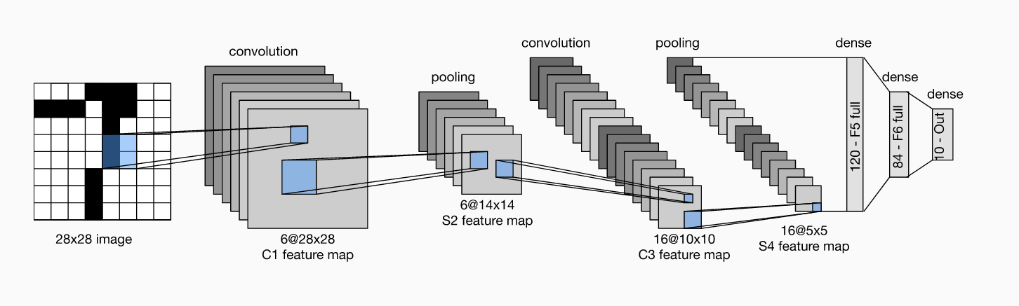
每个卷积块中的基本单元是一个卷积层、一个 sigmoid 激活函数和平均汇聚层。请注意，虽然 ReLU 和最大汇聚层更有效，但它们在20世纪90年代还没有出现。每个卷积层使用 5×5 卷积核和一个 sigmoid 激活函数。这些层将输入映射到多个二维特征输出，通常同时增加通道的数量。第一卷积层有 6 个输出通道，而第二个卷积层有 16 个输出通道。每个 2×2池化操作（步骤2）通过空间下采样将维数减少 4 倍。卷积的输出形状由批量大小、通道数、高度、宽度决定。
为了将卷积块的输出传递给稠密块，我们必须在小批量中展平每个样本。换言之，我们将这个四维输入转换成全连接层所期望的二维输入。这里的二维表示的第一个维度索引小批量中的样本，第二个维度给出每个样本的平面向量表示。LeNet 的稠密块有三个全连接层，分别有 120、84 和 10 个输出。因为我们仍在执行分类，所以输出层的 10 维对应于最后输出结果的数量。

上周房价预测结果

猫狗大战

任务使用lenet作为训练网络没有较好的训练结构，将继续改进。