网络单纯形算法解说【翻译】

转载自 [Tutorial] Network simplex - Codeforces.

网络单纯形算法用于最小成本循环

你好喵！

如果你已经学过单纯形算法和最小成本流算法，也许你听说过这种华丽的东西叫做网络单纯形，它是单纯形算法在计算最小成本循环时的一种专门化/优化。如果你在谷歌搜索中没有找到有趣的结果，或者你的兴趣减退了，你可能会转向其他主题。

不过我没有这样做喵！所以这是关于 最小成本循环 问题的网络单纯形 (NS) 教程。我将描述并表述这个问题，展示它与通常的最小成本流问题的关系，深入解释算法背后的理论，然后推导实现细节。

介绍

在竞争编程中常用于这类任务的算法是基于寻找在 流网络 中进行增广路径的最小成本流算法。流网络是一个有向图，具有指定源 \(s\)、汇 \(t\) 以及带有容量和成本的边。该算法通过在残余网络中找到最便宜的增广路径并逐个饱和它们，从 \(s\) 计算到 \(t\) 的最小成本流。我将称之为 MCF 算法。

现在，我们将在稍微不同的设置下看到的网络单纯形算法，我将其称为 循环网络。循环网络也是一个有向图，其边具有容量和成本，但其节点有一个额外的供给值，表示应该通过节点的流量（在流网络中，此值必须为除 \(s\) 和 \(t\) 以外的每个节点的 \(0\)）。流“进入”一个顶点会增加节点的过剩，而流“退出”一个顶点则会减少它。

没有指定的源或汇。相反，我们有具有 正供给 的节点——可以视为流的 供应者——具有 负供给 的节点——可以视为流的 目的地 或消费；以及具有零供给的节点，作为中间的中转节点。然后，循环就是任意分配流值给边。如果满足所有的供给和容量约束，则循环是 可行的，正如我们稍后将看到的那样。一般而言，存在可行循环的条件是所有节点的供给总和应该等于 \(0\)。

在这个设置下，最小成本循环 只是寻找最小成本 可行循环 的问题。边对循环成本的贡献恰好是通过该边的流量乘以其单元成本，就像在 MCF 算法中一样。

网络单纯形算法是针对这项任务的单纯形算法的专门化。如你将看到的，这个问题可以表述为一个相当简短的线性程序，因此可以通过任何 LP 求解器来解决。然而，常规单纯形算法的直接应用每次枢轴的复杂性为 \(O(VE)\)，并且需要类似的内存来表示表格。通过更仔细地分析线性程序以及其解的结构，我们将找到一种方法，直接在图中执行类似单纯形的算法，以每次枢轴 \(O(V)\) 的期望时间和 \(O(V+E)\) 的内存，导致大多数实例的极快算法。

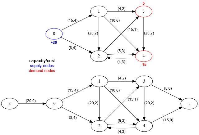
在继续之前，再说几句关于这个循环网络设置的观察。我们可以将循环网络转换为流网络，并将 循环问题 作为 流问题 解决，如下所示。向循环网络添加两个虚拟顶点 \(s\) 和 \(t\)，将 \(s\) 连接到供应节点，将需求节点连接到 \(t\)，两者都使用容量等于相应节点的供给/需求的 \(0\) 成本边。我们刚刚做的是构建一个图，其中任何从 \(s\) 到 \(t\) 的最大流饱和了从 \(s\) 和到 \(t\) 的所有额外边都可以转换为一个可行循环（通过仅移除这些虚拟节点和边）。特别是，最小成本循环问题现在是最小成本流问题，我们可以通过 MCF 算法解决它。

循环网络的一个例子转换，包含 5 个节点，1 个供给节点和 2 个需求节点：

所以如果我们总是可以执行这种归约，为什么需要一个专门的算法呢？首先，MCF 算法无法处理负成本循环，因为其核心算法是 Dijkstra，并且在许多情况下，这种循环的存在并不成问题；而 LP 求解器没有这样的问题，网络单纯形算法也不会。实际上，MCF 算法对负边成本通常存在问题，需要进行特殊初始化与 SPFA/Bellman-Ford，在首次运行时可能非常昂贵。其次，NS 算法相对来说只是极快，因为它免费获得了单纯形算法的所有好处，具体来说，平均上非常少的枢轴数量，与约束的数量成正比。网络单纯形的平均时间复杂性为 \(O(VE)\)，并具有相当好的常数。

本教程的其余部分大致按以下结构进行。首先，我们将把问题正式化为线性程序。然后，我们将研究 角点解 的结构并证明主要正确性定理。这将向我们展示如何在我们的图的上下文中可视化 单纯形算法将会做的事情。接下来，我们将遍历算法必须执行的所有任务，并逐一解决它们，就像我们从头开始设计它一样。在最后，我将提供一个简单的实现，供你在阅读时参考。

前提知识：显然，你需要对一般的流问题设置有所了解，但并不真正需要深入了解任何算法。对线性规划和单纯形算法有良好的理解，有助于你在理论部分轻松跟进。

参考文献：

主要参考来自 MIT OCW。
LEMON 库有一个带有许多优化的参考实现，包括一篇带有基准和一些实现说明的论文。
康奈尔讲义，Williamson。

理论

线性程序表述

设 \(G=(V,E)\) 是一个有向图，节点集为 \(V\)，边集为 \(E\)。让 \(\text{out}(u)\) 和 \(\text{in}(u)\) 分别为从顶点 \(u\) 出发和进入的边的集合。每条边 \(e\) 具有正容量 \(\text{cap}[e]\)、每单位流量的成本 \(\text{cost}[e]\)（没有符号约束），以及待确定的流量量 \(\text{flow}[e]\)。每个顶点 \(u\) 具有一个供给值 \(\text{supply}[u]\)。

我们将通过 \(E\) 维点来表示 \(G\) 中的循环，如 \(x=(\text{flow}[e_1],\ldots,\text{flow}[e_E])\)。

我们可以将最小成本循环问题表述为 \(E\) 变量的线性程序，边流量如下：

\[\begin{align} \text{minimize}\quad & \quad\sum\limits_{e\in E} \text{cost}[e]\cdot\text{flow}[e]\\ \text{subject to}\quad & \\ &(1)\quad \sum\limits_{e\in\text{out}(u)}\text{flow}[e]-\sum\limits_{e\in\text{in}(u)}\text{flow}[e] = \text{supply}[u], \forall u\in V\\ &(2)\quad 0 \leq \text{flow}[e] \leq \text{cap}[e], \forall e\in E\\ \end{align} \]

第一组约束是流量守恒/供给约束。这要求通过顶点 \(u\) 的流量，\(u\) 的过剩，必须等于 \(\text{supply}[u]\)。第二组约束是容量约束。总共有 \(V+E\) 个约束，因此即使使用单纯形法，解决这一问题也确实充满希望。

观察：这个问题永远不会无界，因为 可行区域 被包含在 \((0,\ldots,0)\) 和 \((\text{cap}[e_1],\ldots,\text{cap}[e_E])\) 之间的框中。

现在我们来看一下如何使用单纯形法解决这个线性程序。

寻找一个初始可行解。
1. 如果原点 \(x=(0,\ldots,0)\) 在可行区域内，那么我们就完成了。
  1. 查看图形，如果将 \(\text{flow}[e]=0\) 为每一条边都满足所有约束，那么这是微不足道的，我们就完成了。
2. 否则，原点可能违反了一些约束。向每个这样违反的约束添加一个 人工变量，其初始值为约束的右侧，并解决转换后的 人工问题 以找到一个可行解。
  1. 查看图形，只有供给约束可能被违反。假设它们都被违反，并向每个供给约束/节点添加 \(V\) 个人工变量 \(a_u\)。我们得到了下面显示的转换约束。这种情况几乎总是适用。
优化解：对每当有变量可以进入基时执行一次枢轴。

\[\text{转换的供给约束} \]

\[\begin{cases} \sum\limits_{e\in\text{out}(u)}\text{flow}[e]-\sum\limits_{e\in\text{in}(u)}\text{flow}[e] + a_u = \text{supply}[u] & \text{if}\ \ \text{supply}[u]\geq 0\\ \sum\limits_{e\in\text{out}(u)}\text{flow}[e]-\sum\limits_{e\in\text{in}(u)}\text{flow}[e] - a_u = \text{supply}[u] & \text{if}\ \ \text{supply}[u]< 0\\ \end{cases} \]

如何构建初始单纯形表格？容量约束是不可等式，因此每个约束都得到一个松弛变量，其 \(0\) 成本和初始值为 \(\text{cap}[e]\)。

现在大多数单纯形实现将给所有人工变量分配成本 \(1\)，临时将所有正常变量的成本设置为 \(0\)，并优化以找到人工问题的最小成本解。这必须对可行解存在的情况下具有 \(0\) 成本，这意味着所有人工变量都被设置为 \(0\) 并可以被丢弃。然后，恢复正常变量的原始成本，再次运行算法以找到原始问题的最优解。

我们将采取不同的方法。我们可以为所有人工变量分配 \(\infty\)（待定义）的成本，通常将松弛变量的成本设置为 \(0\)，并保留所有正常变量的成本。如果我们的 \(\infty\) 足够大，那么优化步骤将直接找到原始问题的最优解，或者在没有原始问题的情况下失败。 \(\infty\) 的值必须足够大才能使其工作。

角点是生成树解

单纯形算法沿着可行区域的角点（也称为 极端点）移动。这些点位于可行区域与不可行区域的边界上，并且不是任何其他两个不同的可行点的中点。我们现在将花一些时间研究这些角点在我们的程序中的上下文。

考虑一条边 \(e\)，它通过某一量的 \(\text{flow}[e]\)。我们可以想象一个隐含的反向边，流量为 \(\text{cap}[e]-\text{flow}[e]\)。许多流算法将在残余图中显式表示这些边；而我们在这里不会这样做。

基于这个概念，我们可以将额外的流量 \(\text{cap}[e]-\text{flow}[e]\) 向前推进，通过 \(e\) ，在它饱和之前，同时也可以将流量 \(\text{flow}[e]\) 额外向反向推送，在它 饱和/清空 之前。

考虑原网络中的一个循环 \(C\)，在该循环中，我们被允许沿每条边向前或后走。我们可以通过向前边的流量添加 \(f\)，并向反向边流量减去 \(-f\) 来“发送 \(f\) 流量”或“推动 \(f\) 流量”。供给守恒约束不受影响，因为循环中每个节点追加和减少的流量相等。我们也可以谈论 饱和推动：对于任何循环，存在一个最大这样的 \(f\)，因为任何向前的边不能超过 \(\text{cap}[e]\) 的流量，而被动边不能少于 \(0\) 的流量。所以如果我们饱和这个循环，现在表示我们通过它发送这个最大 \(f\) 流量，至少有一条向前的边 \(e\) 将达到 \(\text{cap}[e]\) 的流量或一条反向边将达到 \(0\) 的流量。在任何情况下，我们可以说该边变得饱和，不再允许沿着循环发送更多流量。

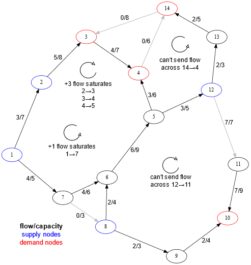
给定一个循环 \(x\)，如果 \(0 < \text{flow}[e] < \text{cap}[e]\)，我们将称一条边 \(e\) 为自由，并且如果它的所有边都是自由的，我们将称一个循环为自由。本质上，我们可以沿着这些边/循环向前或向后推动一定量（可能非常小） \(f\) 的流量。

以下示例显示了左侧的一个自由循环，因为流量可以在其中两个方向上推进。其他两个循环不是自由的，因为它们包含空边或饱和边。

我们将证明网络单纯形的主要定理。

引理 1。任何可行循环 \(x\) 是可行区域的一个角点当且仅当在 \(x\) 中没有自由循环。

证明。

[自由循环 => 不是角点] 设 \(C\) 是一个自由循环。对于足够小的 \(\epsilon>0\)，我们可以沿 \(C\) 发送\(f=\epsilon\)的流量并得到循环 \(x_1\)，但我们也可以发送 \(f=-\epsilon\) 并得到循环 \(x_2\)。我们最终得到了两个不同的可行循环，其在可行区域中的中点为 \(x=\frac{x_1+x_2}{2}\)，因此 \(x\) 不是一个角点。

[不是角点 => 自由循环] 选择不同的可行 \(x_1\) 和 \(x_2\) 使得 \(x=\frac{x_1+x_2}{2}\)。选择任意边 \(e\)。根据 \(x\) 的定义，我们有 \(\text{flow}_x[e]=\frac{\text{flow}_{x_1}[e]+\text{flow}_{x_2}[e]}{2}\)。根据强加在 \(e\) 上的容量约束，我们知道

\[\begin{gather} \text{flow}_x[e]=0 \iff \text{flow}_{x_1}[e]=\text{flow}_{x_2}[e]=0\\ \text{flow}_x[e]=\text{cap}[e] \iff \text{flow}_{x_1}[e]=\text{flow}_{x_2}[e]=\text{cap}[e]\\ \end{gather} \]

现在选择 \(e\) 使得 \(\text{flow}_{x_1}[e]\neq \text{flow}_{x_2}[e]\)。因此 \(e\) 在 \(x\) 中是自由的。

考虑伪循环 \(y=x_1-x_2\)，其中某些边流量可能为负。在 \(y\) 中任何流量非零的边都是 \(x\) 中的自由边。对于循环 \(y\) ，每个顶点的过剩为 \(0\) ，但 \(e\) 的流量非零。如果 \(e\) 从 \(u\) 指向 \(v\) ，则它为 \(v\) 的过剩贡献了非零量。因此，必须存在一条从 \(v\) 出发，指向另一个 \(v_2\) 的边，且流量非零，以抵消 \(e\)。我们可以递归地进行此步骤，找到由非零流量边连接的顶点 \(u,v=v_1,v_2,v_3,\dots\)。由于顶点数量有限，某个顶点最终会重现。这对应于 \(y\) 中的非零流量循环，即 \(x\) 中的自由循环。\(\square\)让我们从以下角度来看引理 1。如果 \(x\) 是一个角点解，且自由边集合无法形成循环，则它必须形成一个森林。那么对于解 \(x\)，我们可以将图的边 \(E\) 划分为三个成对分离的集合 \(T\uplus L\uplus U\)，如下所示：

-\(T\)生成树集——生成树或森林，其边 \(e\in T\) 可以具有任何适当的流量。
-\(L\)下限集——每条边 \(e\in L\) 具有 \(\text{flow}[e]=0\)。
-\(U\)上限集——每条边 \(e\in U\) 具有 \(\text{flow}[e]=\text{cap}[e]\)。

我们明确允许 \(T\) 包含饱和边（带有 \(0\) 或完全流量，其他边则属于 \(L\) 或 \(U\)）。这意味着隔离在 \(T\) 是森林时，当我们将一条边 \(e\) 从 \(L\) 或 \(U\) 移动到 \(T\) 时，划分会保持其属性，而不在 \(T\) 中形成循环。为方便起见，我们可以假设 \(G\) 目前是连接的，因此通过移动一些边始终可以将 \(T\) 转换为一个生成树。即使 \(G\) 是不连通的，算法随后也会对一个连接图进行处理。

反过来，如果循环 \(x\) 可以以这种方式划分，那么它显然 没有自由循环。我们将从此称这些为 生成树解/循环，并记住它们等同于角点。

那么我们为什么要做这些工作呢？现在是时候发挥创造性了！选择一个生成树解 \(x\) ，选择任意不在 \(T\) 中的边 \(e\)。如果我们将 \(e\) 添加到 \(T\)，将形成一个（唯一）循环 \(C\)。如果 \(\text{flow}[e]=0\)，我们可能可以通过 \(C\) 向前推动流量；而如果 \(\text{flow}[e]=\text{cap}[e]\)，我们可能可以通过 \(C\) 向后推动流量。如果我们进行一次这样的 饱和推动，使得另一条边 \(e_{out} \in T\) 变得饱和/清空，我们可以从 \(T\) 中移除 \(e_{out}\)，打破循环，将 \(e\) 添加到 \(T\)，并得到另一个不同的生成树解！

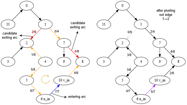
以下图像显示了一个例子。生成树 \(T\) 最初由除 \(e_{in}=(6,10)\) 之外的所有边组成。在识别循环 \(C\) 后，我们看到我们可以通过它推动的最大流量（通过 \(e_{in}\) 向后流量）受限于 \((1,2)\) 和 \((7,8)\)，后者是候选的 \(e_{out}\) 边。

我们刚刚做的是找到一种方法来枢轴从一个生成树解到另一个：只需沿循环发送流量！所选边 \(e\) 是 进入基 的，而变得饱和的边 \(e_{out}\) 是 退出基 的。自然地，解决我们的问题时，我们希望这样的枢轴能 取得进展 并降低循环的成本，因此 循环应具有负成本。请注意，这样的枢轴乐观地可以在 \(O(V)\) 时间内执行，因为这就是受影响的节点和边的数量。将（标准）单纯形算法直接应用于线性程序每个枢轴的消耗时间将是 \(O(VE)\)，并实质上做几乎相同的事情。

通过上述分析，这与通用的单纯形算法完全等价。现在我们要做的就是 重新映射 这些概念回到图形概念中，并利用一些简单的手工图形算法以每个枢轴 \(O(V)\) 时间（或更快的时间）解决问题。

注意，可通过更直接检查单纯形枢轴的动作得出这个结论。我认为以这种方式接近问题为下节中的决策提供了更多动力。

网络单纯形算法

总而言之，这就是我们要做的哪些，给定我们的图 \(G(V,E)\) 设置。

我们希望找到一个初始可行循环，采用某种涉及 \(V\) 人工变量的构建，将其成本设置为无穷大，因为这就是我们在线性程序中所做的。
我们希望快速找到负循环，即带有 “基边” 的循环，该循环位于当前生成树 \(T\) 外面。这些基边是进入基的候选者，且它们的状态是空的或完全饱和。
我们希望有效地维护一棵边的生成树 \(T\)：给定一个进入边 \(e\)，我们必须沿着 \(T\) 确定它的循环 \(C\)，找到可以沿 \(C\) 推送的最大饱和流量 \(f\)，确定退出边 \(t\)，快速更新 \(T\) 的结构和重新计算电势。

最后，就像在单纯形算法中一样，我们通常会有多个候选边进行枢轴，因此我们希望有一个合理的 枢轴策略，即某种聪明的方法可以快速选择优良的边。我们还需要注意不要在生成树解之间循环。

你可以将上述称为“通用网络单纯形”算法。在某种程度上，以下章节描述了我自己的实现。

我们目标为最坏情况的复杂度是每次枢轴 \(O(V)\)，在枢轴选择方面，我们将执行 R中段搜索，正如 LEMON 论文中所述，期望运行时间为 \(O(\sqrt E)\)（可以调整），但最坏情况下运行时间为 \(O(E)\)。

初始可行解

记得我们构建的人工表格吗？我们为每个供给约束创建了 \(V\) 个人工变量，并给每个变量赋值为 \(\infty\)。那 LP 变量在我们的图中的对应是什么呢？

正常变量是图 \(G\) 的边的（流）。
松弛变量是在图 \(G\) 的残余图中的反向边。我们不会显式表示它们。
人工变量... 呃？好吧，我们需要找到初始可行解，而这些变量还未找到，因此我们必须 添加新边！

让我们创建一个特殊的 根节点 \(R\)，并在 \(R\) 和每个其他顶点 \(u\) 之间添加一条 人工边。这些是 \(a_u\) 的体现。

如果 \(u\) 是供给节点（\(\text{supply}[u]>0\)），那么边从 \(u\) 指向 \(R\)，容量为 \(\text{supply}[u]\) ，成本为 \(\infty\)。
如果 \(u\) 是需求节点（\(\text{supply}[u]<0\)），那么边从 \(R\) 指向 \(u\)，容量为 \(-\text{supply}[u]\)，成本也为 \(\infty\)。
如果 \(u\) 是中转节点（\(\text{supply}[u]=0\)），那么边的方向并不重要，但为了方便，我们还是假设是从 \(R\) 指向 \(u\)。

所有这些边都是 初始饱和 的，即对每条人工边 \(a\)，都有 \(\text{flow}[a]=\text{cap}[a]\)。花一点时间来验证这确实是在新图上的可行循环（带有 \(\infty\) 成本）。

减少成本和寻找负循环

假设我们有一条不在生成树边 \(T\) 中的边 \(e\not\in T\)。如果我们将它添加到 \(T\) 中，则会生成一个循环。我们需要一种方法高效地确定这个循环是否具有负成本，并将改善我们的循环。

通常的技巧是计算每个节点 \(u\) 的 电势函数 \(\pi[u]\)，使得对于每个边 \(t=(u,v) \in T\)，减少成本 \(\text{reduced}[t]=\text{cost}[t]+\text{pi}[u]-\text{pi}[v]\) 为 \(0\)（反向边也是如此，因为它具有对称成本）。

假设我们有了这个电势函数和 \(e=(u_{in},v_{in})\)。我们可以沿着生成树追踪路径 \(v_{in}=u_0,u_1,\dots,u_k=u_{in}\)（其中一些是向前的边，一些是反向的边）。然后计算循环 \(C\) 的成本如下（通过 telescoping 总和）：

\[\begin{align} C &= \text{cost}[e] + \sum\limits_{i=0}^{k-1}\text{cost}[(u_i,u_{i+1})] \\ &= \text{cost}[e] + \text{pi}[u_k] - \text{pi}[u_0] + \sum\limits_{i=0}^{k-1}\left(\text{cost}[(u_i,u_{i+1})] + \text{pi}[u_i] - \text{pi}[u_{i+1}]\right) \\ &= \text{cost}[e] + \text{pi}[u_k] + \text{pi}[u_0] \\ &= \text{reduced}[e] \end{align} \]

这意味着我们想要 \(e\in L\) 的前向候选边，其减少成本为负数，以及 \(e\in U\) 的反向候选边，其减少成本为正数。

我们如何计算 \(\text{pi}\)？好吧，我们在节点 \(R\) 上根植了生成树。如果我们设置 \(\text{pi}[R]=0\)，那么 \(\text{pi}[u]\) 则是 \(R\)到\(u\) 沿 \(T\) 的距离，且定义良好，因为恰好存在这样一条路径。记住，沿着反向边遍历边的成本为 \(-\text{cost}[e]\)。

技术上，这条路径包含了一条人工边，其成本为 \(\infty\)。我们如何解决这个问题？

我们可以选择我们的 “\(\infty\)” 为所有正常边的绝对成本之和再加 \(1\)；这样将确保人工边的成本高于任何不包括人工边的循环。

LCA 节点和切割侧

假设我们将边 \(e=(u_{in},v_{in})\) 插入到生成树 \(T\) 中，并且我们将移除一些（尚未知的）边 \(e_{out}\)，该边在推动方向上变得饱和。

生成树以 \(R\) 为根，因此我们可以谈论节点 \(u_{in}\) 和 \(v_{in}\) 的 lca；我们将简化地称之为 lca。我们现在可以在生成树中讨论边 \(e_{out}\) 的侧面： \(e_{out}\) 要么是在 \(u_{in}\) 向 \(lca\) 移动时发现，或是在 \(v_{in}\) 向 \(lca\) 移动时发现（而不是两者皆是）。循环 \(C\) 由 \(v_{in}\) 到 \(lca\) 的路径和从 \(lca\) 到 \(u_{in}\) 的路径组成。这些情况在大多数情况下是对称的；假设 \(e_{out}\) 是在从 \(u_{in}\) 移动时发现的。

为了构建新的生成树，从 \(u_{in}\) 到 \(e_{out}\) 的深度节点的路径将被翻转，即“颠倒过来”；树必须以这样的方式进行转换，使得所有在 \(e_{out}\) 和 \(u\) 之下的节点将成为以 \(u_{in}\) 为根的子树的一部分，而 \(u_{in}\) 的父节点将变为 \(v_{in}\)。

经过这个变换，\(R\) 到在 \(u_{in}\) 的子树中的节点的距离发生改变。经过一些初步计算将证实，对于每个节点，这个距离变化了同样的值 \(\pm \text{reduced}[e]\)，符号取决于沿 \(C\) 的推动方向，我们选择 \(u_{in}\) 还是 \(v_{in}\)。

我们如何找到 \(lca\)？可以有许多方法：我们可以使用环绕双指针技术；我们可以为每个节点维护深度（并在更新时更新它们与电势）；甚至可以使用动态二进制提升！为了简单起见，我建议选择第一种选择，因为它不需要额外的数据结构。

维护生成树 \(T\)

我们如何有效地翻转树并快速访问 \(u_{in}\) 子树中的所有节点（即以真正的 \(O(V)\) 时间）？接下来，我将解释基于链表的实现，而不是线程，这是大多数参考资料建议的内容。

我们将维护每个节点 \(u\) 的父节点 \(\text{parent}[u]\)，以及每个节点 \(u\) 的父边 \(\text{pred}[u]\)（从 \(u\) 到 \(\text{parent}[u]\) 或反向并且在 \(T\) 中的边）。后者使前者有些多余，但不管它！

这样我们就可以轻松地向上移动树，找到 \(lca\)，并访问循环中的所有边。特别是，我们可以找到 \(e_{out}\)。

那么向下呢？我们将维持 \(V+1\) 个双向链表，元素在宇宙 \([0,\ldots,V)+\{R\}\)（顶点）。每个顶点 \(u\) 都有一个匹配的列表，包含它的所有孩子。可以使用 \(2(V+1)\) 大小的两个向量 next 和 prev 来实现这一点。

通过树向下移动并修复电势函数，我们只需迭代 \(u_{in}\) 的双向链表中的顶点，并递归地再次迭代它们。我们可以使用 bfs 或 dfs；这并没有什么区别。

为了翻转路径 \(u_{in} \dots t\)，我们必须修复路径上所有节点的 \(\text{parent}\)，\(\text{pred}\) 和子节点列表。通过记录从 \(u_{in}\) 到 \(u_{out}\) 的路径，修复其向下指针可以在 \(O(V)\) 时间内完成。

如何防止循环 — 选择退出边

当我们尝试针对边 \(e\) 进行枢轴，但因为另一条边 \(t\in C\) 在其上已饱和而未能推动任何流量通过 \(C\)（请记住这是允许的），我们并不更改循环成本或流量。如果在下一次迭代中，我们再次没有改善我们的解决方案，并得到再次选择 \(e\)，那么我们开始循环，并出现无限循环。可能还有多条这样的 \(t\) 被饱和；我们应如何选择其中一条？

我们以与在单纯形算法中防止循环相同的方式防止循环：这些情况基本上是“平局”，我们以某种 字典序 的方式打破平局。请注意，在上述情况下，如果 \(e_{out_1}<e_{out_2}\)，我们可以用 \(e_{out_1}\) 交换 \(e\) 而不是 \(e_{out_2}\)（在我们的边编号系统中）。这等价于 Bland's 规则用于表格行。

LEMON 有另一个想法：假设进入边 \(e\) 从 \(u\) 到 \(v\)。想象循环 \(C\) 从 \(lca\) 开始，沿 \(u\) 通过 \(e\) 向下，并从 \(v\) 回到 \(lca\)。然后，从所有候选退出边中，我们选择在该顺序中出现最后的一条（我们也可以选择第一个）。我想他们已经证明这不会循环。在实践中，这相当于将 \(>\) 交换为 \(\geq\) ，这要优雅得多。

枢轴策略 — 选择进入边

单纯形算法将遍历所有列，选择具有最低负减少成本的边，并在没有找到时终止。这对应于一种枢轴策略，仅检查每条边的减少成本。此过程会花费 \(O(V+E)\) 时间，这对于单纯形算法而言刚好，但如果我们计划在 \(O(V)\) 时间内进行枢轴，则有些次优。这就是 最佳候选 策略：我们检查每条边，并选择最好的一个。

另一种选择是简单地针对找到的第一条边进行枢轴，即 第一候选 策略。显然，这种策略是最快的，但可能选择的进入边并不会显著降低循环成本，从而最终需要更多的枢轴。

在此，我遵循了 LEMON 的实现：在两者之间找到一个中间点。选择某个块大小 \(B\)，并在连续的 \(B\) 条边中以环绕方式运行 最佳候选 策略。如果在 \(B\) 条边之后没有候选者，则再试一次，直到真的穷尽所有边。他们建议 \(B=\sqrt E\)，但 \(B=V\) 应当也能很好地工作。

我个人尚未对这些搜索策略进行基准测试。

就是这样！一旦没有候选进入边，我们就完成了。

实现

关于实现的最后几点：

通过适当地调整每条边 \(e\) 的流向 lower 和 upper 界限，我们可以轻松地添加对此的支持，使用 upper-lower 作为整个算法中 \(e\) 的容量，并在结束时撤消调整。
如果在算法结束时一些人工边仍然存在流量，则问题是不可行的。更具体地说，如果最初从 \(R\) 引出的边有 \(S\) 总流量，而在算法结束时它们的流量为 \(0 \leq F \leq S\)，那么 \(S-F\) 本质上就是通过循环网络的“最大流”。

问题与应用

正如在第一部分讨论的那样，这对于 MCF 算法在相同场景中是替代方案。因此，问题主要是最小成本流问题。只要问题不涉及增广路径的明确定义或对总流量/循环成本的限制，它都应该可以使用 NS 来解决。

~ 我会在找到更多问题时添加到这里喵~

Network Simplex Algorithm for Minimum Cost Circulation

Hello!

If you've learned the simplex algorithm and a minimum cost flow algorithm, perhaps you've also heard about this fancy thing called network simplex which is supposed to be a specialization/optimization of the simplex algorithm for computing a minimum cost circulation. If your Google search didn't turn up any interesting results or your interest faded, you might have moved on to other subjects.

Well I didn't! So this is a tutorial on network simplex (NS) for the minimum cost circulation problem. I'll describe and formulate the problem, show how it relates to the usual minimum cost flow problem, explain the theory behind the algorithm in-depth, and then derive the implementation details.

Introduction

The algorithm commonly used in competitive programming for this sort of task is a minimum cost flow algorithm based on finding augmenting paths in a flow network. A flow network is a directed graph with a designated source\(s\), a sink\(t\), and edges with capacities and costs. This algorithm computes minimum cost flows from\(s\)to\(t\)by finding the cheapest augmenting paths in the residual network and saturating them, one at a time. I will call this the MCF algorithm.

Now, the network simplex algorithm we'll see here works in a slightly different setting, on what I'll call a circulation network. A circulation network is also a directed graph whose edges have capacities and costs, but whose nodes have an additional supply value, indicating the amount of flow that should pass through the node (in a flow network this value must be\(0\)for every node except\(s\)and\(t\)). Flow "entering" a vertex increases the excess of the node, and flow "exiting" a vertex decreases it.

There is no designated source or sink. Instead we have nodes with positive supply — which can be seen as suppliers of flow — nodes with negative supply — which can be seen as destinations or consumers of flow; and nodes with zero supply, which are intermediate transshipment nodes. A circulation is then an arbitrary assignment of flow values to the edges. The circulation is feasible if it meets all the supply and capacity constraints, as we'll see below. In general, the sum of the supplies of all nodes should be\(0\)for a feasible circulation to exist.

Under this setting, minimum cost circulation is simply the problem of finding the minimum cost feasible circulation. The contribution of an edge to the circulation cost is just the amount of flow going through that edge multiplied by its unit cost, just like in the MCF algorithm.

The network simplex algorithm is a specialization of the simplex algorithm for this task. As you'll see below, this problem can be formulated as a pretty short linear program, and thus solved by any LP solver. However, a direct application of the usual simplex algorithm has a complexity of\(O(VE)\)per pivot, and a similar memory requirement to represent the tableau. By analyzing the linear program more carefully and the structure of its solutions, we will find a way to perform a simplex-style algorithm directly in the graph and achieve\(O(V)\)expected time per pivot with\(O(V+E)\)memory, leading to an extremely fast algorithm for most instances.

A few more observations about this circulation network setup before we proceed. We can convert a circulation network into a flow network, and solve circulation problems as flow problems, as follows. Add two dummy vertices\(s\)and\(t\)to the circulation network, link\(s\)to supply nodes, demand nodes to\(t\), both using edges of\(0\)cost and capacity equal to the supply/demand at the respective nodes. What we have just done is built a graph where any maximum flow from\(s\)to\(t\)that saturates all the extra edges out of\(s\)and into\(t\)can be converted into a feasible circulation (by just removing these dummy nodes and edges). In particular, the minimum cost circulation problem is now the minimum cost flow problem, which we can solve with the MCF algorithm.

Example transformation of a circulation network with 5 nodes, 1 supply node and 2 demand nodes:

So if we can always perform this reduction, why do we need a specialized algorithm? First, the MCF algorithm cannot handle negative cost cycles since its core algorithm is Dijkstra, and in many cases the presence of such cycles is not an issue; LP solvers have no such problems, and so neither will the NS algorithm. In fact, the MCF algorithm has issues with negative edge costs in general, requiring a special initialization with SPFA/Bellman-Ford on the first run that can be very expensive. Secondly, the NS algorithm is just lightning fast in comparison, as it gets all of the benefits of the simplex algorithm for free, namely a very low number of pivots on average, proportional to the number of constraints. Network simplex will run with a time complexity of\(O(VE)\)on average, and with a pretty good constant.

The rest of the tutorial is structured roughly as follows. First, we'll formalize the problem as a linear program. Then we'll study the structure of corner points solutions and prove the main correctness theorem. This will show us how to visualize what the simplex algorithm would do in the context of our graph. Then we'll go over all the tasks the algorithm must perform and solve them one by one, as if we were designing it from scratch. At the end, I'll provide a simple implementation that you can also follow while reading.

Prerequisites: Obviously, you need to be familiar with the setting of flow problems in general, but no in-depth knowledge of any algorithm is actually required. A good understanding of linear programming and the simplex algorithm is needed to follow along in the theory section comfortably.

References:

Main reference from MIT OCW.
The LEMON library has a reference implementation with many optimizations, and includes a paper with benchmarks and some implementation notes.
Cornell Lecture notes, Williamson.

Theory

Linear Program Formulation

Let\(G=(V,E)\)be a directed graph with node set\(V\)and edge set\(E\). Let\(\text{out}(u)\)and\(\text{in}(u)\)be the set of edges exiting and entering vertex\(u\), respectively. Every edge\(e\)has a positive capacity\(\text{cap}[e]\), a cost per unit of flow\(\text{cost}[e]\)(no constraints on sign), and a flow amount\(\text{flow}[e]\)to be determined. Every vertex\(u\)has a supply value\(\text{supply}[u]\).

We will represent a circulation in\(G\)by\(E\)-dimensional points such as\(x=(\text{flow}[e_1],...,\text{flow}[e_E])\).

We can formalize the minimum cost circulation problem as a linear program over\(E\)variables, the edge flows, as follows:

\[\begin{align} \text{minimize}\quad & \quad\sum\limits_{e\in E} \text{cost}[e]\cdot\text{flow}[e]\\ \text{subject to}\quad & \\ &(1)\quad \sum\limits_{e\in\text{out}(u)}\text{flow}[e]-\sum\limits_{e\in\text{in}(u)}\text{flow}[e] = \text{supply}[u], \forall u\in V\\ &(2)\quad 0 \leq\text{flow}[e] \leq\text{cap}[e], \forall e\in E\\ \end{align} \]

The first set of constraints are the flow conservation/supply constraints. These require the amount of flow passing through vertex\(u\), the excess of\(u\), to be exactly equal to\(\text{supply}[u]\). The second set of constraints are the capacity constraints. There are exactly\(V+E\)constraints, so there really is hope of solving this efficiently, even with the simplex method.

Observation: The problem is never unbounded, as the feasible region is contained in the box between\((0,...,0)\)and\((\text{cap}[e_1],...,\text{cap}[e_E])\).

So now let's see how we would solve this linear program using the simplex method.

Find an initial feasible solution.
1. If the origin\(x=(0,...,0)\)is in the feasible region then we are done.
  1. Looking at the graph, if setting\(\text{flow}[e]=0\)for every edge satisfies all constraints, then this is trivial and we are done.
2. Otherwise, the origin might violate some constraints. Add one artificial variable to each such constraint whose initial value is the right-hand side of the constraint, and solve the transformed artificial problem to find a feasible solution.
  1. Looking at the graph, only the supply constraints might be violated. Just suppose they are all violated, and add\(V\)artificial variables\(a_u\), one to each supply constraint/vertex. We get the transformed constraints shown below. This case virtually always applies.
Optimize the solution: Perform a pivot for as long as there are variables that can enter the basis.

\[\text{Transformed supply constraints} \]

How does the initial simplex tableau get built? The capacity constraints are inequalities, so they each get a slack variable with\(0\)cost and initial value\(\text{cap}[e]\).

Now most simplex implementations will assign a cost of\(1\)to all artificial variables, temporarily set the cost of all normal variables to\(0\), and optimize to find a minimum cost solution of the artificial problem. This must have\(0\)cost for a feasible solution to exist, meaning all artificial variables were set to\(0\)and can be discarded. Then the original costs of the normal variables are restored, and the algorithm is run again to find the optimal solution of the original problem.

We will do something different. We can assign a cost of\(\infty\)(to be defined) to all artificial variables,\(0\)cost to slack variables as usual, and retain the cost of all normal variables. If our\(\infty\)is large enough, then the optimize step will just find an optimal solution to the original problem outright, or fail if one doesn't exist. The value of\(\infty\)must be large enough for this to work.

Corner Points are Spanning Tree Solutions

The simplex algorithm moves along corner points of the feasible region (also called extreme points). These are points that lie on the boundary between the feasible and infeasible region, and are not the halfway point of any other two distinct feasible points. We will now take a moment to study these corner points in the context of our program.

Consider an edge\(e\)which has a certain amount of\(\text{flow}[e]\)passing through it. We can imagine an implicit backward edge that has\(\text{cap}[e]-\text{flow}[e]\)flow going through it. Many flow algorithms will represent these edges explicitly in a residual graph; we will not do it here.

With this notion, we can push\(\text{cap}[e]-\text{flow}[e]\)extra flow forward along\(e\)before it saturates, and we can push\(\text{flow}[e]\)extra flow backward along\(e\)before it saturates/empties.

Consider a cycle\(C\)in the original network, one where we are allowed to go forward or backward along each edge. We can "send\(f\)flow" or "push\(f\)flow" along this cycle by adding\(f\)to the flow of forward edges and\(-f\)to the flow of backward edges in\(C\). The supply conservation constraints are unaffected, since the same amount of flow was added and subtracted from every node in the cycle. We can also talk about saturating pushes: for any cycle there is one maximum such\(f\), as any forward edge cannot go over\(\text{cap}[e]\)flow and backward edges cannot go under\(0\)flow. So if we saturate this cycle, which means we send this maximum\(f\)flow through it, at least one forward edge\(e\)will reach\(\text{cap}[e]\)flow or one backward edge will reach\(0\)flow. In either case we can say such an edge became saturated and did not allow more flow to be sent along the cycle.

Given a circulation\(x\), we'll call an edge\(e\)free if\(0<\text{flow}[e]<\text{cap}[e]\), and we'll call a cycle free if all of its edges are free. Essentially, we can push a (possibly very small) amount\(f\)of flow forwards or backwards along these edges/cycles.

The following example shows a free cycle on the left, as flow can be pushed through it in either direction. The other two cycles are not free, as they contain empty or saturated edges.

We'll now prove the main theorem behind network simplex.

Lemma 1. Any feasible circulation\(x\)is a corner point of the feasible region iff there is no free cycle in\(x\).

Proof.

[free cycle => not corner point] Let\(C\)be a free cycle. For a sufficiently small\(\epsilon>0\)we can send\(f=\epsilon\)flow around\(C\)and get circulation\(x_1\), but we can also send\(f=-\epsilon\)and get circulation\(x_2\). We end up with two distinct feasible circulations whose midpoint in the feasible region is\(x=\frac{x_1+x_2}{2}\), therefore\(x\)is not a corner point.

[not corner point => free cycle] Pick distinct feasible\(x_1\)and\(x_2\)such that\(x=\frac{x_1+x_2}{2}\). Pick any edge\(e\). By definition of\(x\)we have\(\text{flow}_x[e]=\frac{\text{flow}_{x_1}[e]+\text{flow}_{x_2}[e]}{2}\). Due to the capacity constraints enforced on\(e\), we know

\[\begin{gather} \text{flow}_x[e]=0 \iff \text{flow}_{x_1}[e]=\text{flow}_{x_2}[e]=0\\ \text{flow}_x[e]=\text{cap}[e] \iff \text{flow}_{x_1}[e]=\text{flow}_{x_2}[e]=\text{cap}[e]\\ \end{gather} \]

Now pick\(e\)such that\(\text{flow}_{x_1}[e]\neq \text{flow}_{x_2}[e]\). Then\(e\)is free in\(x\).

Consider the pseudo-circulation\(y=x_1-x_2\), where some of the edge flows may be negative. Any edge in\(y\)with non-zero flow is a free edge in\(x\). The excess at every vertex is\(0\)for the circulation\(y\), but\(e\)has non-zero flow. If\(e\)goes out from\(u\)to\(v\), then it contributes a non-zero amount to the excess at\(v\). Hence there must be at least one edge out of\(v\)to some other\(v_2\)with non-zero flow, to counterbalance\(e\). We can induct this step to find vertices\(u,v=v_1,v_2,v_3,\dots\)connected by non-zero flow edges in\(y\). Since there are only a finite number of vertices, some vertex eventually repeats. This corresponds to a non-zero flow cycle in\(y\), i.e. a free cycle in\(x\).\(\square\)Let's look at lemma 1 the following way. If\(x\)is a corner point solution, and the set of free edges cannot form cycles, it must form a forest. Then for the solution\(x\), we can partition the graph's edges\(E=T\uplus L\uplus U\)into three pairwise disjoint sets, as follows:

-\(T\)Spanning Tree Set — A spanning tree or forest, whose edges\(e\in T\)can have any adequate flow.
-\(L\)Lower Set — Every edge\(e\in L\)has\(\text{flow}[e]=0\).
-\(U\)Upper Set — Every edge\(e\in U\)has\(\text{flow}[e]=\text{cap}[e]\).

We explicitly allow\(T\)to contain saturated edges (with\(0\)or full flow, that would otherwise belong to\(L\)or\(U\)). This means the partitioning maintains its properties when\(T\)is a forest and we move an edge\(e\)in\(L\)or\(U\)to\(T\)without creating a cycle in\(T\). For convenience, we can assume\(G\)is connected for now, so turning\(T\)into a spanning tree by moving some edges is always possible. The algorithm later will do its work on a connected graph even if\(G\)is disconnected.

Conversely, if a circulation\(x\)can be partitioned this way, then it clearly has no free cycles. We will henceforth call these spanning tree solutions/circulations, and remember they are equivalent to corner points.

So why did we do all this work? Now is the time to get creative! Pick a spanning tree solution\(x\)and pick any edge\(e\not\in T\). If we added\(e\)to\(T\)we would form a (unique) cycle\(C\). If\(\text{flow}[e]=0\)we might be able to push flow forward through\(C\), and if\(\text{flow}[e]=\text{cap}[e]\)we might be able to push flow backward through\(C\). If we make one such saturating push, such that another edge\(e_{out}\in T\)becomes saturated/empty, we can remove\(e_{out}\)from\(T\), break the cycle, add\(e\)to\(T\), and get another, different, spanning tree solution!

The following image shows an example. The spanning tree\(T\)is initially made up of all the edges shown except\(e_{in}=(6,10)\). After identifying the cycle\(C\), we see that the maximum amount of flow we can push through it (which goes backwards through\(e_{in}\)) is limited by\((1,2)\)and\((7,8)\), which are the candidate\(e_{out}\)edges.

What we have just done here is find a way to pivot from one spanning tree solution to another: just send flow along a cycle! The chosen edge\(e\)is entering the basis, while the edge\(e_{out}\)which became saturated is exiting the basis. Naturally, to solve our problem, we want such a pivot to make progress and reduce the cost of the circulation, so the cycle should have negative cost. Notice that such a pivot can optimistically be performed in\(O(V)\)time, as that is the number of nodes and edges affected. A straightforward application of the (standard) simplex algorithm to the linear program would take\(O(VE)\)for each pivot, and do essentially the same thing.

By the analysis above, this is completely equivalent to a generic simplex algorithm. All we have to do now is map these concepts back into graph concepts, and solve the problem with some simple handcrafted graph algorithms in\(O(V)\)time per pivot (or better).

Noted, it is possible to arrive at this conclusion by a more direct inspection of the actions of a simplex pivot. I think approaching the problem this way grants more motivation for the decisions made in the next section.

The Network Simplex Algorithm

To sum up, this is what we want to do, given our graph\(G(V,E)\)setup.

We want to find an initial feasible circulation, employing some sort of construction involving\(V\)artificial variables with infinite cost, since that is what we did in the linear program.
We want to find negative cycles quickly, cycles with a "base edge" outside of the current spanning tree\(T\). These base edges are candidates for entering the basis and are either empty or fully saturated.
We want to maintain a spanning tree\(T\)of edges efficiently: given an entering edge\(e\), we must identify its cycle\(C\)along\(T\), find the maximum saturating flow\(f\)that can be pushed along\(C\), identify the exiting edge\(t\), update\(T\)'s structure, and recompute potentials quickly.

Finally, just like in the simplex algorithm, we will generally have multiple candidate edges to pivot on, so we want a decent pivoting strategy, i.e. some clever way to select good edges quickly. We will also need to take care not to cycle between spanning tree solutions.

You could call the above the "generic network simplex" algorithm. To some extent, the following sections describe my own implementation.

We target a complexity of\(O(V)\)per pivot in the worst-case, and for pivot selection we will perform a block search as described in the LEMON paper, with a desired runtime of\(O(\sqrt E)\)(can be tuned), but worst-case runtime of\(O(E)\).

Initial Feasible Solution

Remember the artificial tableau we built? We created\(V\)artificial variables for each of the supply constraints and gave each of them a cost of\(\infty\). What do the LP variables correspond to in our graph?

The normal variables are the (flow of)\(G\)'s edges.
The slack variables are the backward edges in the residual graph of\(G\). We will not represent them explicitly.
The artificial variables... huh? Well, we need to find an initial feasible solution, and these are nowhere to be found just yet, so we must add new edges for them!

Let's create a special root node\(R\), and add an artificial edge between\(R\)and every other vertex\(u\). These are the incarnations of\(a_u\).

If\(u\)is a supply node (\(\text{supply}[u]>0\)), then the edge is oriented from\(u\)to\(R\), has capacity\(\text{supply}[u]\), and\(\infty\)cost.
If\(u\)is a demand node (\(\text{supply}[u]<0\)), then the edge is oriented from\(R\)to\(u\), has capacity\(-\text{supply}[u]\), and also\(\infty\)cost.
If\(u\)is a transshipment node (\(\text{supply}[u]=0\)) then it doesn't matter which way the edge goes, but we want one for convenience; let's treat these as supply nodes.

All these edges are initially saturated, i.e.\(\text{flow}[a]=\text{cap}[a]\)for every artificial edge\(a\). Take a moment to verify this is indeed a feasible circulation on the new graph (with\(\infty\)cost).

Reduced Costs and Finding Negative Cycles

Suppose we have a non-spanning tree edge\(e\not\in T\). If we add it to\(T\)it creates a cycle. We need a way to determine, efficiently, whether this cycle has negative cost and would improve our circulation.

The usual trick is computing a potential function\(\pi[u]\)for every node\(u\)such that for every edge\(t=(u,v)\in T\), the reduced cost\(\text{reduced}[t]=\text{cost}[t]+\text{pi}[u]-\text{pi}[v]\)is\(0\)(and the same is true of the backward edge, since it has symmetric cost).

Suppose we have this potential function and\(e=(u_{in},v_{in})\). We can trace out the path\(v_{in}=u_0,u_1,\dots,u_k=u_{in}\)along the spanning tree (some of these are forward and some are backward edges). The cost of the cycle\(C\)in the direction of\(e\)is then computed as (by a telescoping sum):

This means we want forward candidate edges\(e\in L\)with negative reduced cost, and backward candidate edges\(e\in U\)with positive reduced cost.

How do we compute\(\text{pi}\)? Well, we rooted the spanning tree on the node\(R\). If we set\(\text{pi}[R]=0\), then\(\text{pi}[u]\)is simply the distance from\(R\)to\(u\)along\(T\), and is well defined as there is exactly one such path. Remember that the cost of traversing an edge\(e\)backwards is\(-\text{cost}[e]\).

Technically this path includes an artificial edge with\(\infty\)cost. How do we address this?

We can pick for our "\(\infty\)" the sum of absolute costs of all the normal edges, plus\(1\); this will guarantee that the artificial edges have higher cost than any cycle not including an artificial edge.

The LCA Node and the Cut Side

Suppose we're inserting edge\(e=(u_{in},v_{in})\)into the spanning tree\(T\), and we're going to remove some (yet unknown) edge\(e_{out}\)which became saturated along the direction of the push.

The spanning tree is rooted at\(R\), so we can talk about the lca of nodes\(u_{in}\)and\(v_{in}\); we'll call it simply\(lca\). Now we can talk about the side of\(e_{out}\)in the spanning tree: either\(e_{out}\)is found walking up from\(u_{in}\)to\(lca\), or it is found walking up from\(v_{in}\)to\(lca\)(and not both). The cycle\(C\)is made up of the path from\(v_{in}\)to\(lca\)and from\(lca\)to\(u_{in}\). These cases are symmetric for the most part; assume\(e_{out}\)is found walking from\(u_{in}\).

To build the new spanning tree, the path from\(u_{in}\)to\(e_{out}\)'s deeper node will be everted, i.e. "flipped on its head"; the tree must be transformed in such a way that all the nodes below\(e_{out}\)and\(u\)will become part of a subtree rooted at\(u_{in}\), and\(u_{in}\)'s parent will become\(v_{in}\).

After this transformation, the distance of\(R\)to the nodes in the subtree of\(u_{in}\)changed. Some back of the envelope calculations will show it changed by the same value\(\pm\ \text{reduced}[e]\)for every node, with the sign depending on the orientation of the push along\(C\)and whether we picked\(u_{in}\)or\(v_{in}\).

How do we actually find\(lca\)? There are many ways: we can use the wraparound two pointers technique; we can maintain depths for every node (and update them along with the potentials); and we can even use dynamic binary lifting! For simplicity, I suggest the first option, as it requires no extra data structures.

Maintaining the Spanning Tree\(T\)

How do we actually evert the tree and visit all the nodes in the subtree of\(u_{in}\)quickly afterwards (that is, in true\(O(V)\)time)? In the following, I will explain an implementation based on linked lists, rather than threads, which is what is suggested in most references.

We will maintain the parent vertex\(\text{parent}[u]\)of every node\(u\), and also the parent edge\(\text{pred}[u]\)for every node\(u\)(the edge that goes from\(u\)to\(\text{parent}[u]\)or vice-versa and is in\(T\)). The latter makes the former somewhat redundant, but whatever!

This way we can go up the tree easily, find\(lca\), and visit all the edges in the cycle. In particular, we can find\(e_{out}\).

How about going down? We will maintain\(V+1\)doubly linked lists with elements in the universe\([0,...,V)+\{R\}\)(the vertices). Each vertex\(u\)has a matching list containing all of its children. This can be implemented with two vectors next and prev of size\(2(V+1)\).

To go down the tree and fix the potential function, we simply iterate over the vertices in the doubly linked list of\(u_{in}\), and iterate those again recursively. We can do it with bfs or dfs; it does not matter.

To evert the path\(u_{in}\dots t\)we must fix the\(\text{parent}\),\(\text{pred}\), and children lists of all the nodes on the path. This can be performed in linear time by recording the path from\(u_{in}\)to\(u_{out}\)and fixing the pointers downwards.

How to Prevent Cycling — Choosing Exiting Arc

When we try to pivot on an edge\(e\)and end up pushing no flow through\(C\)because another edge\(t\in C\)on it was already saturated (remember this is allowed), we do not change the circulation cost or flow. If in the next iterations, we once again do not improve our solution, and end up picking\(e\)again, then we start cycling, and we have an infinite loop. There may also be several such\(t\)that get saturated; how do we pick one?

We prevent cycling the same way we prevent it in the simplex algorithm: these situations are basically "ties", and we break the ties in some lexicographic way. Notice that in the situation above, we can exchange\(e\)for\(e_{out_1}\)over\(e_{out_2}\)if\(e_{out_1}<e_{out_2}\)(in our edges' numbering system). This is equivalent to Bland's tie breaking rule for tableau rows.

LEMON had another idea: suppose the entering edge\(e\)goes from\(u\)to\(v\). Imagine the cycle\(C\)starting at\(lca\), going down to\(u\)through\(e\)and up from\(v\)back to\(lca\). Then, from all candidate exiting edges, we pick the one that appears last in this order (we could also pick the first). I suppose they have proven this will not cycle. In practice, this amounts to exchanging a\(>\)for a\(\geq\), which is quite more elegant.

Pivoting Strategy — Choosing Entering Arc

The simplex algorithm would run through all the columns and pick the one with the lowest negative reduced cost and terminate if none is found. This corresponds to a pivoting strategy that just checks the reduced cost of every edge. This takes\(O(V+E)\)time, which is just fine for the simplex algorithm, but a bit sub-optimal if we plan to pivot in\(O(V)\)time. This is the best-candidate strategy: we check every edge and pick the best one.

Another option would be to simply pivot on the first edge found, called the first-candidate strategy. This strategy is obviously the fastest, but might pick entering edges that don't reduce the circulation cost by a lot, requiring more pivots overall.

I followed the LEMON implementation here: use a middle ground between the two. Pick some block size\(B\), and run the best-candidate strategy among\(B\)consecutive edges in a wraparound fashion. If after\(B\)edges it finds no candidate, it just tries again, and again, until it has actually exhausted all edges. They suggest\(B=\sqrt E\), but\(B=V\)should work fine as well.

I have not personally benchmarked any of these search strategies against each other.

And that's it! We are done once there are no candidate entering edges.

Implementation

Some final points about the implementation:

We can easily add support for lower and upper bounds for the flow along an edge\(e\), by adjusting the supplies of the nodes by the value of lower, using upper-lower as the capacity of\(e\)throughout the algorithm, and at the ending undoing the adjustment.
If at the end of the algorithm some artificial edges still have flow on them, the problem is infeasible. More specifically, if the edges leading out of\(R\)initially had\(S\)total flow and at the end of the algorithm they have\(0 \leq F \leq S\)total flow, then\(S-F\)is essentially the "maximum flow" through the circulation network.

Problems and Applications

As discussed in the first section, this is an alternative to the MCF algorithm in the same scenarios. So the problems are mostly minimum cost flow problems. As long as the problem does not involve the explicit consideration of augmenting paths or a bound on the total flow/circulation cost, it should be solvable with NS.

~ I'll add more problems here as I find them.

posted @ 2025-01-23 21:44 zhiyin123123 阅读(91) 评论(0) 收藏举报

刷新页面返回顶部

zhiyin123