第四次作业:卷积神经网络 part3
代码练习
HybridSN
三维卷积部分:
conv1:(1, 30, 25, 25), 8个 7x3x3 的卷积核 ==>(8, 24, 23, 23) conv2:(8, 24, 23, 23), 16个 5x3x3 的卷积核 ==>(16, 20, 21, 21) conv3:(16, 20, 21, 21),32个 3x3x3 的卷积核 ==>(32, 18, 19, 19)
接下来要进行二维卷积,因此把前面的 32*18 reshape 一下,得到 (576, 19, 19)
二维卷积:(576, 19, 19) 64个 3x3 的卷积核,得到 (64, 17, 17)
接下来是一个 flatten 操作,变为 18496 维的向量,
接下来依次为256,128节点的全连接层,都使用比例为0.4的 Dropout,
最后输出为 16 个节点,是最终的分类类别数。
class HybridSN(nn.Module):
  def __init__(self):
    super(HybridSN,self).__init__()
    self.conv3d1 = nn.Conv3d(1,8,kernel_size=(7,3,3),stride=1,padding=0)
    self.bn1 = nn.BatchNorm3d(8)
    self.conv3d2 = nn.Conv3d(8,16,kernel_size=(5,3,3),stride=1,padding=0)
    self.bn2 = nn.BatchNorm3d(16)
    self.conv3d3 = nn.Conv3d(16,32,kernel_size=(3,3,3),stride=1,padding=0)
    self.bn3 = nn.BatchNorm3d(32)
    self.conv2d4 = nn.Conv2d(576,64,kernel_size=(3,3),stride=1,padding=0)
    self.bn4 = nn.BatchNorm2d(64)
    self.fc1 = nn.Linear(18496,256)
    self.fc2 = nn.Linear(256,128)
    self.fc3 = nn.Linear(128,16)
    self.dropout = nn.Dropout(0.4)

  def forward(self,x):
    out = F.relu(self.bn1(self.conv3d1(x)))
    out = F.relu(self.bn2(self.conv3d2(out)))
    out = F.relu(self.bn3(self.conv3d3(out)))
    out = F.relu(self.bn4(self.conv2d4(out.reshape(out.shape[0],-1,19,19))))
    out = out.reshape(out.shape[0],-1)
    out = F.relu(self.dropout(self.fc1(out)))
    out = F.relu(self.dropout(self.fc2(out)))
    out = self.fc3(out)
    return out
# 对高光谱数据 X 应用 PCA 变换
def applyPCA(X, numComponents):
    newX = np.reshape(X, (-1, X.shape[2]))
    pca = PCA(n_components=numComponents, whiten=True)
    newX = pca.fit_transform(newX)
    newX = np.reshape(newX, (X.shape[0], X.shape[1], numComponents))
    return newX

# 对单个像素周围提取 patch 时,边缘像素就无法取了,因此,给这部分像素进行 padding 操作
def padWithZeros(X, margin=2):
    newX = np.zeros((X.shape[0] + 2 * margin, X.shape[1] + 2* margin, X.shape[2]))
    x_offset = margin
    y_offset = margin
    newX[x_offset:X.shape[0] + x_offset, y_offset:X.shape[1] + y_offset, :] = X
    return newX

# 在每个像素周围提取 patch ,然后创建成符合 keras 处理的格式
def createImageCubes(X, y, windowSize=5, removeZeroLabels = True):
    # 给 X 做 padding
    margin = int((windowSize - 1) / 2)
    zeroPaddedX = padWithZeros(X, margin=margin)
    # split patches
    patchesData = np.zeros((X.shape[0] * X.shape[1], windowSize, windowSize, X.shape[2]))
    patchesLabels = np.zeros((X.shape[0] * X.shape[1]))
    patchIndex = 0
    for r in range(margin, zeroPaddedX.shape[0] - margin):
        for c in range(margin, zeroPaddedX.shape[1] - margin):
            patch = zeroPaddedX[r - margin:r + margin + 1, c - margin:c + margin + 1]
            patchesData[patchIndex, :, :, :] = patch
            patchesLabels[patchIndex] = y[r-margin, c-margin]
            patchIndex = patchIndex + 1
    if removeZeroLabels:
        patchesData = patchesData[patchesLabels>0,:,:,:]
        patchesLabels = patchesLabels[patchesLabels>0]
        patchesLabels -= 1
    return patchesData, patchesLabels

def splitTrainTestSet(X, y, testRatio, randomState=345):
    X_train, X_test, y_train, y_test = train_test_split(X, y, test_size=testRatio, random_state=randomState, stratify=y)
    return X_train, X_test, y_train, y_test

# 地物类别
class_num = 16
X = sio.loadmat('Indian_pines_corrected.mat')['indian_pines_corrected']
y = sio.loadmat('Indian_pines_gt.mat')['indian_pines_gt']

# 用于测试样本的比例
test_ratio = 0.90
# 每个像素周围提取 patch 的尺寸
patch_size = 25
# 使用 PCA 降维,得到主成分的数量
pca_components = 30

print('Hyperspectral data shape: ', X.shape)
print('Label shape: ', y.shape)

print('\n... ... PCA tranformation ... ...')
X_pca = applyPCA(X, numComponents=pca_components)
print('Data shape after PCA: ', X_pca.shape)

print('\n... ... create data cubes ... ...')
X_pca, y = createImageCubes(X_pca, y, windowSize=patch_size)
print('Data cube X shape: ', X_pca.shape)
print('Data cube y shape: ', y.shape)

print('\n... ... create train & test data ... ...')
Xtrain, Xtest, ytrain, ytest = splitTrainTestSet(X_pca, y, test_ratio)
print('Xtrain shape: ', Xtrain.shape)
print('Xtest  shape: ', Xtest.shape)

# 改变 Xtrain, Ytrain 的形状,以符合 keras 的要求
Xtrain = Xtrain.reshape(-1, patch_size, patch_size, pca_components, 1)
Xtest  = Xtest.reshape(-1, patch_size, patch_size, pca_components, 1)
print('before transpose: Xtrain shape: ', Xtrain.shape)
print('before transpose: Xtest  shape: ', Xtest.shape)

# 为了适应 pytorch 结构,数据要做 transpose
Xtrain = Xtrain.transpose(0, 4, 3, 1, 2)
Xtest  = Xtest.transpose(0, 4, 3, 1, 2)
print('after transpose: Xtrain shape: ', Xtrain.shape)
print('after transpose: Xtest  shape: ', Xtest.shape)


""" Training dataset"""
class TrainDS(torch.utils.data.Dataset):
    def __init__(self):
        self.len = Xtrain.shape[0]
        self.x_data = torch.FloatTensor(Xtrain)
        self.y_data = torch.LongTensor(ytrain)
    def __getitem__(self, index):
        # 根据索引返回数据和对应的标签
        return self.x_data[index], self.y_data[index]
    def __len__(self):
        # 返回文件数据的数目
        return self.len

""" Testing dataset"""
class TestDS(torch.utils.data.Dataset):
    def __init__(self):
        self.len = Xtest.shape[0]
        self.x_data = torch.FloatTensor(Xtest)
        self.y_data = torch.LongTensor(ytest)
    def __getitem__(self, index):
        # 根据索引返回数据和对应的标签
        return self.x_data[index], self.y_data[index]
    def __len__(self):
        # 返回文件数据的数目
        return self.len

# 创建 trainloader 和 testloader
trainset = TrainDS()
testset  = TestDS()
train_loader = torch.utils.data.DataLoader(dataset=trainset, batch_size=128, shuffle=True, num_workers=2)
test_loader  = torch.utils.data.DataLoader(dataset=testset,  batch_size=128, shuffle=False, num_workers=2)
训练一下~
这里注意一下 net.train() 和net.eval()
官方文档这么说的
eval()
Sets the module in evaluation mode.This has any effect only on certain modules. See documentations of particular modules for details of their behaviors in training/evaluation mode, if they are affected, e.g. Dropout, BatchNorm, etc.
train(mode=True)
Sets the module in training mode.This has any effect only on certain modules. See documentations of particular modules for details of their behaviors in training/evaluation mode, if they are affected, e.g.Dropout, BatchNorm, etc.
引用下知乎的一个回答
model的eval方法主要是针对某些在train和predict两个阶段会有不同参数的层。比如Dropout层和BN层
Dropout在train时随机选择神经元 而predict要使用全部神经元并且要乘一个补偿系数
BN在train时每个batch做了不同的归一化因此也对应了不同的参数,相应predict时实际用的参数是每个batch下参数的移动平均。
torch为了方便大家,设计这个eval方法就是让我们可以不用手动去针对这些层做predict阶段的处理(也可以叫evaluation阶段,所以这个方法名才是eval)
这也就是说,如果模型中用了dropout或bn,那么predict时必须使用eval 否则结果是没有参考价值的,不存在选择的余地。
作者:蔺笑天
链接:https://www.zhihu.com/question/363144860/answer/951669576
来源:知乎
著作权归作者所有。商业转载请联系作者获得授权,非商业转载请注明出处。
# 使用GPU训练,可以在菜单 "代码执行工具" -> "更改运行时类型" 里进行设置
device = torch.device("cuda:0" if torch.cuda.is_available() else "cpu")

# 网络放到GPU上
net = HybridSN().to(device)
criterion = nn.CrossEntropyLoss()
optimizer = optim.Adam(net.parameters(), lr=0.001)


# 开始训练
total_loss = 0
net.train()
for epoch in range(100):
    for i, (inputs, labels) in enumerate(train_loader):
        inputs = inputs.to(device)
        labels = labels.to(device)
        # 优化器梯度归零
        optimizer.zero_grad()
        # 正向传播 + 反向传播 + 优化
        outputs = net(inputs)
        loss = criterion(outputs, labels)
        loss.backward()
        optimizer.step()
        total_loss += loss.item()
    print('[Epoch: %d]   [loss avg: %.4f]   [current loss: %.4f]' %(epoch + 1, total_loss/(epoch+1), loss.item()))

print('Finished Training')
测试下
count = 0
net.train()
# 模型测试
for inputs, _ in test_loader:
inputs = inputs.to(device)
outputs = net(inputs)
outputs = np.argmax(outputs.detach().cpu().numpy(), axis=1)
if count == 0:
y_pred_test = outputs
count = 1
else:
y_pred_test = np.concatenate( (y_pred_test, outputs) )
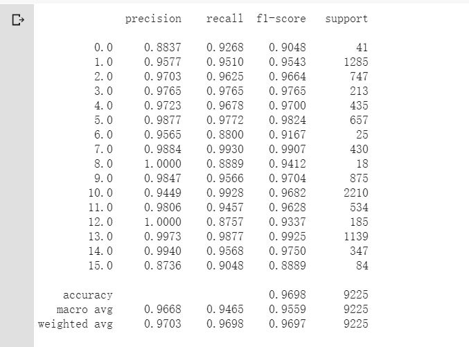
# 生成分类报告
classification = classification_report(ytest, y_pred_test, digits=4)
print(classification)
Hybrid中添加SENet
主要参考了 https://zhuanlan.zhihu.com/p/65459972
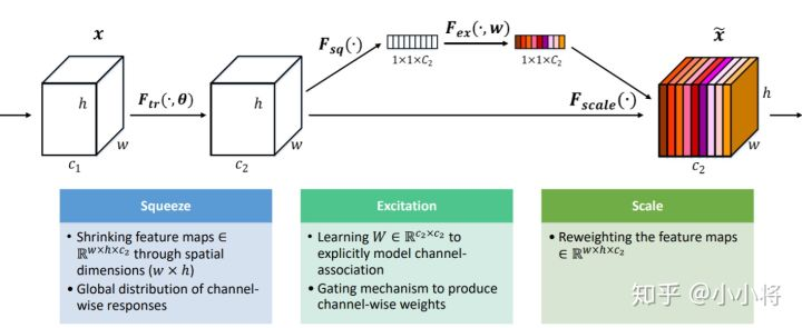
定义SENet
class SE(nn.Module):
  def __init__(self,channel,reduction=16):
    super(SE,self).__init__()
    self.pool = nn.AdaptiveAvgPool2d(1)#Squeeze
    self.fc = nn.Sequential( #excitation
        nn.Linear(channel,channel//reduction,bias=False),
        nn.ReLU(True),
        nn.Linear(channel // reduction, channel, bias=False),
        nn.Sigmoid()
    )
  def forward(self,x):
    out = self.pool(x)
    out = out.view(out.shape[0],-1)
    out = self.fc(out)
    out = out.view(x.shape[0],x.shape[1],1,1)
    return x*out
- 缩减倍数reduction是一个超参数,在不同的深度的layer中,可以选择调整不同的缩减比例来提高你的网络性能。
Hybrid中添加SENet
class HybridSN(nn.Module):
  def __init__(self):
    super(HybridSN,self).__init__()
    self.conv3d1 = nn.Conv3d(1,8,kernel_size=(7,3,3),stride=1,padding=0)
    self.bn1 = nn.BatchNorm3d(8)
    self.conv3d2 = nn.Conv3d(8,16,kernel_size=(5,3,3),stride=1,padding=0)
    self.bn2 = nn.BatchNorm3d(16)
    self.conv3d3 = nn.Conv3d(16,32,kernel_size=(3,3,3),stride=1,padding=0)
    self.bn3 = nn.BatchNorm3d(32)
    self.conv2d4 = nn.Conv2d(576,64,kernel_size=(3,3),stride=1,padding=0)
    self.SElayer = SE(64,16)
    self.bn4 = nn.BatchNorm2d(64)
    self.fc1 = nn.Linear(18496,256)
    self.fc2 = nn.Linear(256,128)
    self.fc3 = nn.Linear(128,16)
    self.dropout = nn.Dropout(0.4)

  def forward(self,x):
    out = F.relu(self.bn1(self.conv3d1(x)))
    out = F.relu(self.bn2(self.conv3d2(out)))
    out = F.relu(self.bn3(self.conv3d3(out)))
    out = F.relu(self.bn4(self.conv2d4(out.reshape(out.shape[0],-1,19,19))))
    out = self.SElayer(out)
    out = out.reshape(out.shape[0],-1)
    out = F.relu(self.dropout(self.fc1(out)))
    out = F.relu(self.dropout(self.fc2(out)))
    out = self.fc3(out)
    return out
训练测试
# 网络放到GPU上
net = HybridSN().to(device)

criterion = nn.CrossEntropyLoss()
optimizer = optim.Adam(net.parameters(), lr=0.001)
scheduler = optim.lr_scheduler.ReduceLROnPlateau(optimizer, 'min',verbose=True,factor=0.9,min_lr=1e-6)

# 开始训练
total_loss = 0
net.train()
for epoch in range(100):
    for i, (inputs, labels) in enumerate(train_loader):
        inputs = inputs.to(device)
        labels = labels.to(device)
        # 优化器梯度归零
        optimizer.zero_grad()
        # 正向传播 + 反向传播 + 优化
        outputs = net(inputs)
        loss = criterion(outputs, labels)
        loss.backward()
        optimizer.step()
        scheduler.step(loss)
        total_loss += loss.item()
        nn.ReLU()
    print('[Epoch: %d]   [loss avg: %.4f]   [current loss: %.4f]' %(epoch + 1, total_loss/(epoch+1), loss.item()))

print('Finished Training')
net.eval()
count = 0
# 模型测试
for inputs, _ in test_loader:
    inputs = inputs.to(device)
    outputs = net(inputs)
    outputs = np.argmax(outputs.detach().cpu().numpy(), axis=1)
    if count == 0:
        y_pred_test =  outputs
        count = 1
    else:
        y_pred_test = np.concatenate( (y_pred_test, outputs) )

# 生成分类报告
classification = classification_report(ytest, y_pred_test, digits=4)
print(classification)
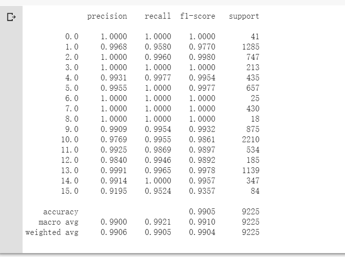
准确率达到了99%,比不加入SENet提升了3%左右~
SE模块主要为了提升模型对channel特征的敏感性,这个模块是轻量级的,而且可以应用在现有的网络结构中,只需要增加较少的计算量就可以带来性能的提升
视频学习
语义分割中的自注意力机制和低秩重重建
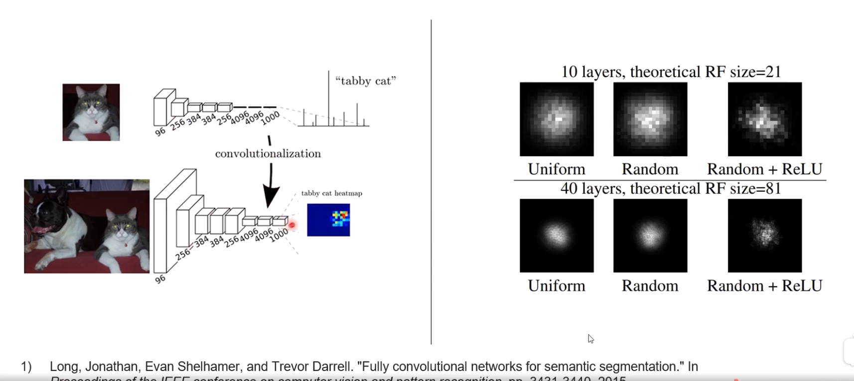
FUlly convolutional networks
图像分类 通过一系列卷积 avg pooling得到1x1的大小,再经过fc层得出分类
FCN将图片分辨率加大,avg pooling后得到NxN大小的图片,提高感知域,得到预测结果;但是实际感知域还是很小,而语义分割需要很大的感知域。全卷积网络无法实现这一要求
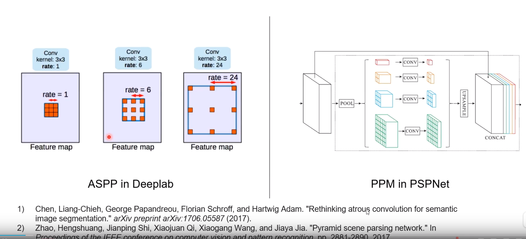
- ASPP in Deeplab
- 为了提高有效感知域,通过带洞卷积(Dilated Convolution)分成多路,来收集不同远近的信息
Nonlocal Neural Networks
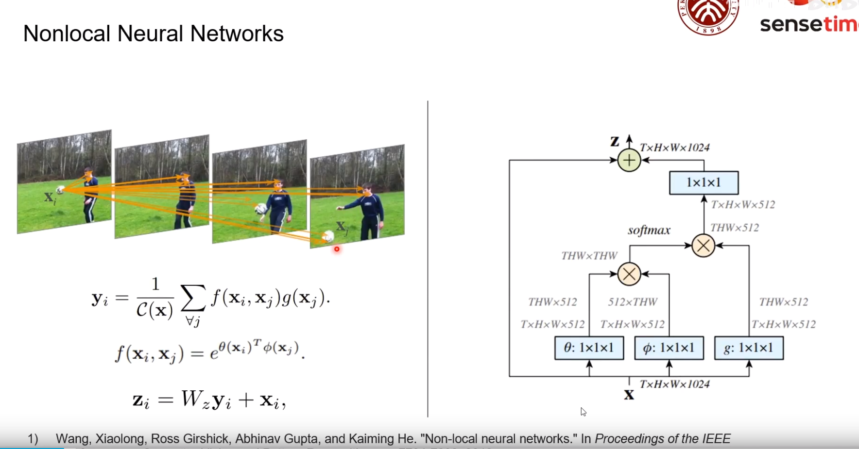
为了推测一个物体的信息,需要建立此位置与其他各个点的信息。
f(xi,xj) 建模了xi与xj的关系;g(xj)是对要参考的像素的变换

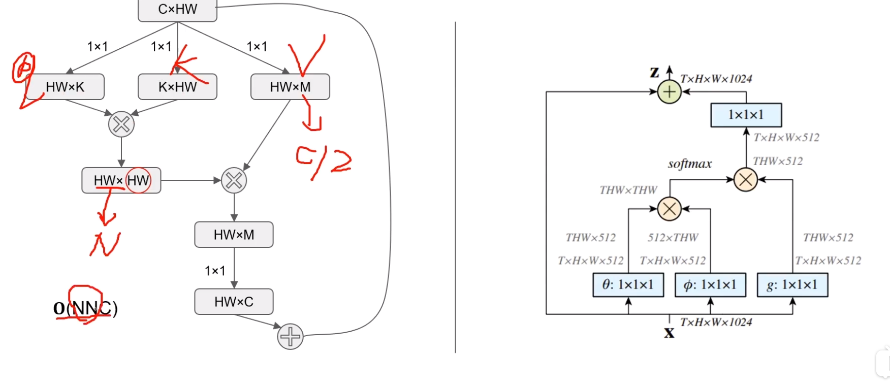
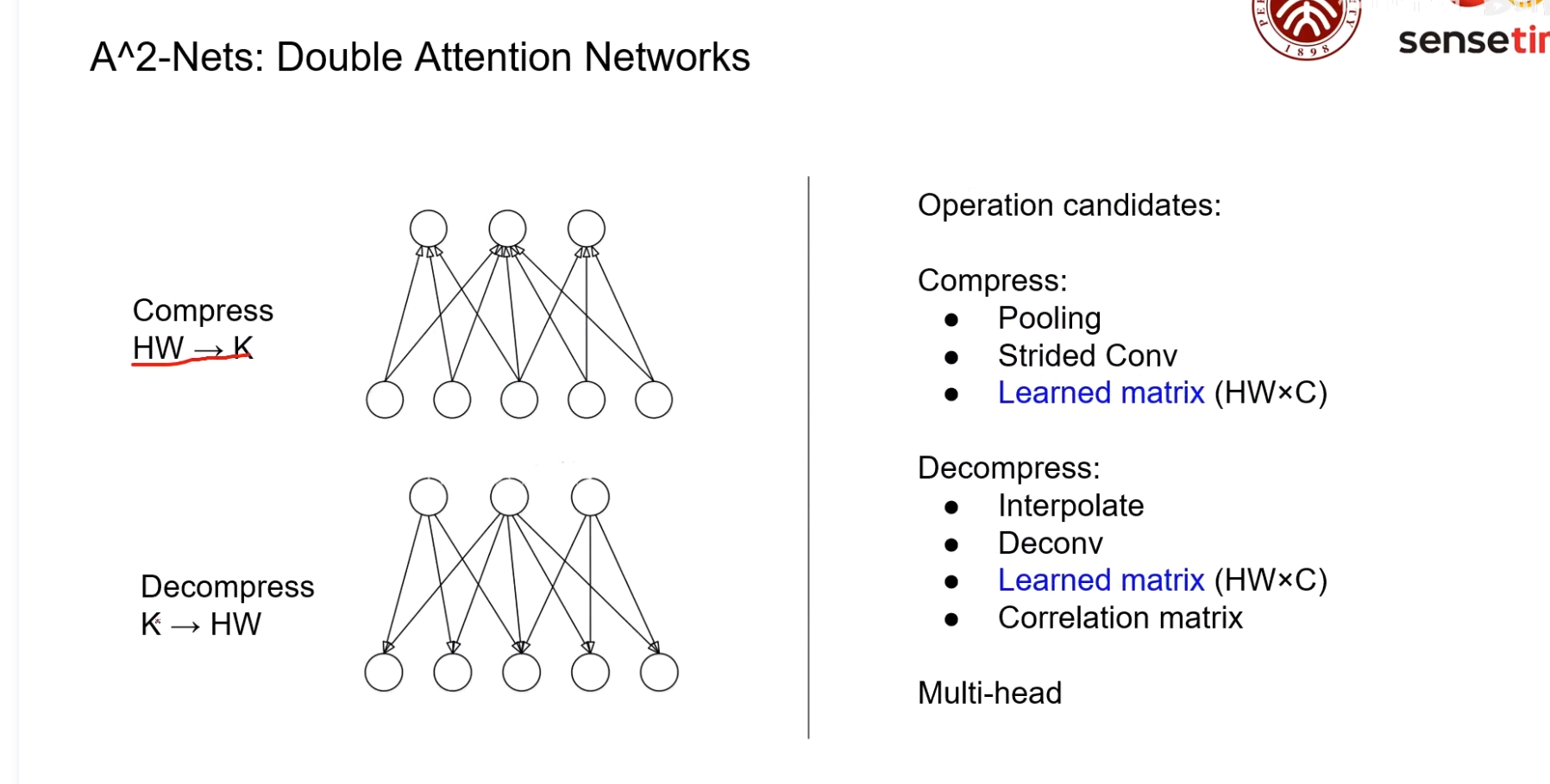
A^2 Net


通过这种方式可以将O(NNC)降低至O(NCC) (C远小于N)
图像语义分割前沿进展

左半部分是类ResNet的网络结构,这种结构有一定的多尺度表达能力,但是还是不够
右半部分在左侧基础上将输入分成了多组进行分组卷积,可以更好的提出不同尺度的信息,而且计算量比左半部分更小
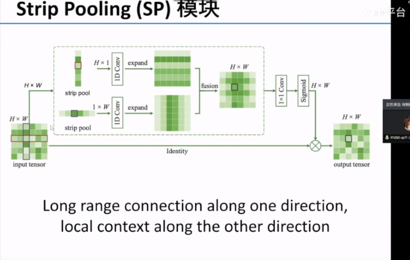
通过带状池化(Strip Pooling)在语义分割时可以在一个方向上获得全局的信息,同时在另一个方向上获得细节信息。
