8.4 8.5 8.7 8.8 8.9

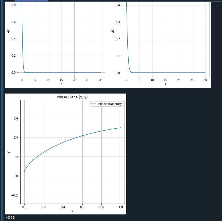
8.4

点击查看代码

import numpy as np
import matplotlib.pyplot as plt
from scipy.integrate import solve_ivp

def system(t, state):
    x, y = state
    dxdt = -x*3 - y
    dydt = x - y*3
    return [dxdt, dydt]

t_span = (0, 30)
y0 = [1, 0.5]

sol = solve_ivp(system, t_span, y0, t_eval=np.linspace(t_span[0], t_span[1], 1000))

x = sol.y[0]
y = sol.y[1]
t = sol.t

plt.figure(figsize=(12, 6))

plt.subplot(1, 2, 1)
plt.plot(t, x, label='x(t)')
plt.xlabel('t')
plt.ylabel('x(t)')
plt.title('x(t) vs t')
plt.legend()
plt.grid(True)

plt.subplot(1, 2, 2)
plt.plot(t, y, label='y(t)')
plt.xlabel('t')
plt.ylabel('y(t)')
plt.title('y(t) vs t')
plt.legend()
plt.grid(True)

plt.figure(figsize=(6, 6))
plt.plot(x, y, label='Phase Trajectory')
plt.xlabel('x')
plt.ylabel('y')
plt.title('Phase Plane (x, y)')
plt.legend()
plt.grid(True)
plt.axis('equal')

plt.tight_layout()
plt.show()

print("3010")

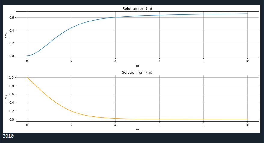
7.5

点击查看代码

import numpy as np
import matplotlib.pyplot as plt
from scipy.integrate import solve_ivp

def model(t, y):
    f, df_dm, d2f_dm2, T, dT_dm = y
    d3f_dm3 = -3*f*d2f_dm2 + 2*(df_dm)**2 - T
    d2T_dm2 = -2.1*f*dT_dm
    return [df_dm, d2f_dm2, d3f_dm3, dT_dm, d2T_dm2]

y0 = [0, 0, 0.68, 1, -0.5]

t_span = (0, 10)
t_eval = np.linspace(t_span[0], t_span[1], 1000)

sol = solve_ivp(model, t_span, y0, t_eval=t_eval, method='RK45')

f = sol.y[0]
T = sol.y[3]

plt.figure(figsize=(12, 6))

plt.subplot(2, 1, 1)
plt.plot(sol.t, f, label='f(m)')
plt.xlabel('m')
plt.ylabel('f(m)')
plt.title('Solution for f(m)')
plt.grid(True)

plt.subplot(2, 1, 2)
plt.plot(sol.t, T, label='T(m)', color='orange')
plt.xlabel('m')
plt.ylabel('T(m)')
plt.title('Solution for T(m)')
plt.grid(True)

plt.tight_layout()
plt.show()

print("3010")

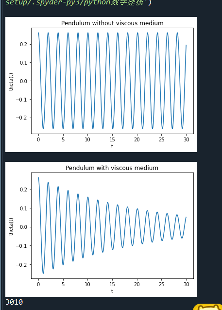
8.7

点击查看代码

import numpy as np
import matplotlib.pyplot as plt
from scipy.integrate import odeint

def pendulum_ode_1(y, t, g, l):
    theta, omega = y
    dydt = [omega, -g / l * np.sin(theta)]
    return dydt

l = 1
g = 9.8
theta_0 = 15 / 180 * np.pi
y0 = [theta_0, 0]
t = np.linspace(0, 30, 1000)
sol_1 = odeint(pendulum_ode_1, y0, t, args=(g, l))

plt.plot(t, sol_1[:, 0])
plt.xlabel('t')
plt.ylabel('theta(t)')
plt.title('Pendulum without viscous medium')
plt.show()

def pendulum_ode_2(y, t, g, l, lambda_):
    theta, omega = y
    dydt = [omega, -g / l * np.sin(theta) - lambda_ / l * omega]
    return dydt

lambda_ = 0.1
y0 = [theta_0, 0]
sol_2 = odeint(pendulum_ode_2, y0, t, args=(g, l, lambda_))

plt.plot(t, sol_2[:, 0])
plt.xlabel('t')
plt.ylabel('theta(t)')
plt.title('Pendulum with viscous medium')
plt.show()
print("3010")

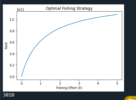
8.8

点击查看代码

import numpy as np
from scipy.integrate import odeint
import matplotlib.pyplot as plt


# 定义参数
b3 = 0.5 * 1.109 * 10**5
b4 = 1.109 * 10**5
s = lambda n: 1.22 * 10**11 / (1.22 * 10**11 + n)
d = 0.8
w3 = 17.86
w4 = 22.99
q3 = 0.42
q4 = 1
E = 1  # 初始捕捞努力量，后面会进行优化


def fish_model(x, t):
    x1, x2, x3, x4 = x
    n = b3 * x3 + b4 * x4
    dx1dt = (b3 * x3 + b4 * x4) * s(n) - d * x1
    dx2dt = x1 * (1 - d) - d * x2
    dx3dt = x2 * (1 - d) - d * x3 - q3 * E * x3
    dx4dt = x3 * (1 - d) - d * x4 - q4 * E * x4
    return [dx1dt, dx2dt, dx3dt, dx4dt]


# 初始鱼群数量
x0 = [1000, 1000, 1000, 1000]
t = np.linspace(0, 10, 1000)
sol = odeint(fish_model, x0, t)


# 计算捕捞量
def calculate_yield(x, E):
    x3, x4 = x[2], x[3]
    return (w3 * q3 * E * x3 + w4 * q4 * E * x4)


# 寻找最优捕捞努力量（简单示例，实际可能需要更复杂的优化算法）
Es = np.linspace(0, 5, 100)
yields = []
for e in Es:
    E = e
    sol = odeint(fish_model, x0, t)
    x_end = sol[-1]
    yield_value = calculate_yield(x_end, E)
    yields.append(yield_value)

optimal_E_index = np.argmax(yields)
optimal_E = Es[optimal_E_index]


# 绘制结果
plt.plot(Es, yields)
plt.xlabel('Fishing Effort (E)')
plt.ylabel('Yield')
plt.title('Optimal Fishing Strategy')
plt.show()
print("3010")

8.9

点击查看代码

r=0.0036
N=360
Q=400000
x=round((1+r)**N*Q*r/((1+r)**N-1),2)
xt=x*N
print('月还款额为：',x);print('总还款额为：',xt)
print("3010")