图像求导及模糊

在很多应用中，图像强度的变化情况是非常重要的信息。强度的变化可以灰度图像的\(x\)和\(y\)方向导数\(I_x\)和\(I_y\)进行描述。图像的梯度向量为\(\nabla I = [I_x, I_y]^T\)。梯度有两个重要属性，一个是梯度的大小：

\[| \nabla I | = \sqrt{I_x^2+I_y^2} \]

它描述了图像强度变化的强弱，另一个是梯度的角度：

\[\alpha = arctan2(I_y, I_x) \]

描述了图像中每个像素点上强度变化最大的方向。我们可以使用离散近似的方式来计算图像的导数。图像导数大多数可以通过卷积简单地实现：

\[I_x = I*D_x \ 和\ I_y = I*D_y \]

对于\(D_x\)和\(D_y\)，通常选择Priwitt滤波器：

\[D_x = \left[ \begin{matrix} -1 & 0 & 1 \\ -1 & 0 & 1 \\ -1 & 0 & 1 \end{matrix} \right] 和D_y=\left[ \begin{matrix} -1 & -1 & -1 \\ 0 & 0 & 0 \\ 1 & 1 & 1 \end{matrix} \right] \]

或者Sobel滤波器:

\[D_x = \left[ \begin{matrix} -1 & 0 & 1 \\ 2 & 0 & 2 \\ -1 & 0 & 1 \end{matrix} \right] 和D_y=\left[ \begin{matrix} -1 & -2 & -1 \\ 0 & 0 & 0 \\ 1 & 2 & 1 \end{matrix} \right] \]

上面两种计算图像导数的方法存在一些缺陷：滤波器的尺度需要随着图像分辨率的变化而变化。为了在图像噪声方面更稳健，以及在任意尺度上计算导数，我们可以使用高斯导数滤波器：

\[I_x = I*G_{\sigma x} 和 I_y = I*G_{\sigma y} \]

其中，\(G_{\sigma x}\) 和 \(G_{\sigma y}\) 表示 \(G_\sigma\) 在\(x\)和\(y\)方向上的导数，\(G_\sigma\) 为标准差为\(\sigma\)的高斯函数。

样例演示

from scipy.ndimage import filters
from PIL import Image
import numpy as np
import matplotlib.pyplot as plt


class ScipyFilter:
    def __init__(self, path: str):
        self.img = np.array(Image.open(path))
        self.grayImg = np.array(Image.open(path).convert('L'))
        self.Ix = np.zeros(self.grayImg.shape)
        self.Iy = np.zeros(self.grayImg.shape)
        self.manitude = np.zeros(self.grayImg.shape)

    def cal_derivatives_sobel(self):
        """
        使用sobel滤波器计算导数
        :return:
        """
        filters.sobel(self.grayImg, 1, self.Ix)
        filters.sobel(self.grayImg, 0, self.Iy)
        self.manitude = np.sqrt(self.Ix**2 + self.Iy**2)

    def cal_derivatives_prewitt(self):
        """
        使用prewitt滤波器计算导数
        :return:
        """
        filters.prewitt(self.grayImg, 1, self.Ix)
        filters.prewitt(self.grayImg, 0, self.Iy)
        self.manitude = np.sqrt(self.Ix**2 + self.Iy**2)

    def cal_derivatives_gaussian(self, sigma):
        """
        计算图像高斯导数
        :param img: 图像数据
        :param sigma: 标准差
        :return:
        """
        filters.gaussian_filter(self.grayImg, (sigma, sigma), (0, 1), self.Ix)
        filters.gaussian_filter(self.grayImg, (sigma, sigma), (1, 0), self.Iy)

    def plot(self):
        # 绘图
        plt.figure()
        plt.gray()
        plt.subplot(221).set_title("original img")
        plt.imshow(self.grayImg)
        plt.axis('off')
        plt.subplot(222).set_title('x-directional derivative')
        plt.imshow(self.Ix)
        plt.axis('off')
        plt.subplot(223).set_title('y-directional derivative')
        plt.imshow(self.Iy)
        plt.axis('off')
        plt.subplot(224).set_title("gradient magnitude")
        plt.imshow(self.manitude)
        plt.axis('off')
        plt.show()


if __name__ == '__main__':
    img_path = "./imgs/3.jpg"
    sc = ScipyFilter(img_path)
    sc.cal_derivatives_sobel()
    sc.plot()
    sc.cal_derivatives_prewitt()
    sc.plot()
    sc.cal_derivatives_gaussian(3)
    sc.plot()
    sc.cal_derivatives_gaussian(5)
    sc.plot()

结果演示

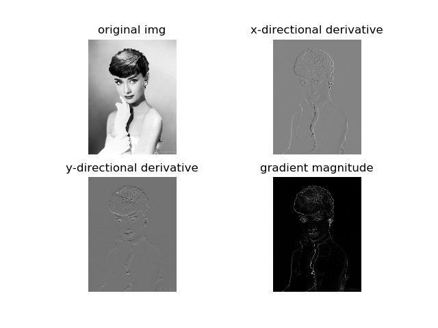
sobel滤波

prewitt滤波

gaussian滤波，标准差设置为3

gaussian滤波，标准差设置为5

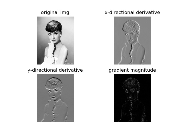
在图像中，正导数显示为亮的像素，负导数显示为暗的像素。灰色区域表示导数的值接近零。

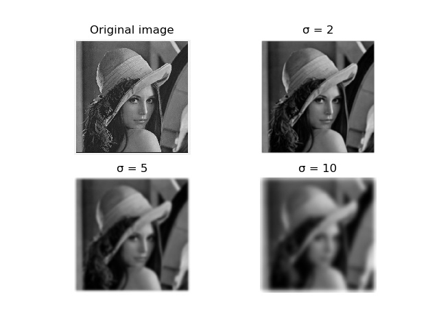
图像高斯模糊

from PIL import Image
import numpy as np
from scipy.ndimage import filters


img = Image.open(r"girl.jpg").convert('L')
img = np.array(img)
img2 = filters.gaussian_filter(img, 2)
img3 = filters.gaussian_filter(img, 5)
img4 = filters.gaussian_filter(img, 10)

结果演示

更多参考上一篇