卷积神经网络的引入1--MLP再图像像素平移之后的局限性

！！！ 本文重现的实验来自V Kishore Ayyadevara 著作的Modern Computer Vision with PyTorch (Second Edition) 一书，以下论述仅代表个人理解，如想体验原汁原味，强烈建议阅读原书。
Fully Connected Neural Network在目标识别的局限，通过以下代码实现

# Import libraries and download data
from torchvision import datasets
from pathlib import Path
import torch
import matplotlib.pyplot as plt
%matplotlib inline
import numpy as np
from torch.utils.data import Dataset, DataLoader
import torch.nn as nn
from torch.optim import SGD, Adam
import seaborn as sns

# Download FashionMNIST dataset
data_folder = Path('./data/fashion_mnist')
data_folder.mkdir(parents=True, exist_ok=True)
fmnist = datasets.FashionMNIST(data_folder, download=True, train=True)

# Load training data
tr_images = fmnist.data
tr_targets = fmnist.targets

# Load validation data
val_fmnist = datasets.FashionMNIST(data_folder, download=True, train=False)
val_images = val_fmnist.data
val_targets = val_fmnist.targets

# Set device
device = 'cuda' if torch.cuda.is_available() else 'cpu'

# Define Dataset class
class FMNISTDataset(Dataset):
    def __init__(self, x, y):
        x = x.float()/255
        x = x.view(-1,28*28)
        self.x, self.y = x, y 
    def __getitem__(self, ix):
        x, y = self.x[ix], self.y[ix]        
        return x.to(device), y.to(device)
    def __len__(self): 
        return len(self.x)

# Define model function
def get_model():
    model = nn.Sequential(
        nn.Linear(28 * 28, 1000),
        nn.ReLU(),
        nn.Linear(1000, 10)
    ).to(device)

    loss_fn = nn.CrossEntropyLoss()
    optimizer = Adam(model.parameters(), lr=1e-3)
    return model, loss_fn, optimizer

# Define training function
def train_batch(x, y, model, opt, loss_fn):
    prediction = model(x)
    batch_loss = loss_fn(prediction, y)
    batch_loss.backward()
    optimizer.step()
    optimizer.zero_grad()
    return batch_loss.item()

# Define accuracy function
def accuracy(x, y, model):
    with torch.no_grad():
        prediction = model(x)
    max_values, argmaxes = prediction.max(-1)
    is_correct = argmaxes == y
    return is_correct.cpu().numpy().tolist()

# Define data loading function
def get_data():     
    train = FMNISTDataset(tr_images, tr_targets)     
    trn_dl = DataLoader(train, batch_size=32, shuffle=True)
    val = FMNISTDataset(val_images, val_targets)     
    val_dl = DataLoader(val, batch_size=len(val_images), shuffle=True)
    return trn_dl, val_dl

# Define validation loss function
def val_loss(x, y, model, loss_fn):
    with torch.no_grad():
        prediction = model(x)
    val_loss = loss_fn(prediction, y)
    return val_loss.item()

# Get data and model
trn_dl, val_dl = get_data()
model, loss_fn, optimizer = get_model()

# Training loop
train_losses, train_accuracies = [], []
val_losses, val_accuracies = [], []
for epoch in range(5):
    print(epoch)
    train_epoch_losses, train_epoch_accuracies = [], []
    for ix, batch in enumerate(iter(trn_dl)):
        x, y = batch
        batch_loss = train_batch(x, y, model, optimizer, loss_fn)
        train_epoch_losses.append(batch_loss)        
    train_epoch_loss = np.array(train_epoch_losses).mean()

    for ix, batch in enumerate(iter(trn_dl)):
        x, y = batch
        is_correct = accuracy(x, y, model)
        train_epoch_accuracies.extend(is_correct)
    train_epoch_accuracy = np.mean(train_epoch_accuracies)

    for ix, batch in enumerate(iter(val_dl)):
        x, y = batch
        val_is_correct = accuracy(x, y, model)
        validation_loss = val_loss(x, y, model, loss_fn)
    val_epoch_accuracy = np.mean(val_is_correct)

    train_losses.append(train_epoch_loss)
    train_accuracies.append(train_epoch_accuracy)
    val_losses.append(validation_loss)
    val_accuracies.append(val_epoch_accuracy)

# Display sample image
ix = 24300
plt.imshow(tr_images[ix], cmap='gray')
plt.title(fmnist.classes[tr_targets[ix]])
plt.show()

# Prepare image for prediction
img = tr_images[ix]/255.
img = img.view(28*28)
img = img.to(device)

# Get prediction
np_output = model(img).cpu().detach().numpy()
print(np.exp(np_output)/np.sum(np.exp(np_output)))

# Show target label
print(f"Target: {tr_targets[ix]}")

# Test translation invariance
preds = []
for px in range(-5,6):
    img = tr_images[ix]/255.
    img = img.view(28, 28)
    img2 = np.roll(img, px, axis=1)
    plt.imshow(img2)
    plt.show()
    img3 = torch.Tensor(img2).view(28*28).to(device)
    np_output = model(img3).cpu().detach().numpy()
    preds.append(np.exp(np_output)/np.sum(np.exp(np_output)))

# Visualize translation results
fig, ax = plt.subplots(1,1, figsize=(12,10))
plt.title('Probability of each class for various translations')
sns.heatmap(np.array(preds), annot=True, ax=ax, fmt='.2f', 
            xticklabels=fmnist.classes, 
            yticklabels=[str(i)+str(' pixels') for i in range(-5,6)], 
            cmap='gray')

import numpy as np
import torch
import matplotlib.pyplot as plt
import seaborn as sns

# 假设模型和数据都已加载好
# 这里 ix 是你选择的图片索引
ix = 24300
img = tr_images[ix] / 255.

preds = []  # 存放每次平移后的概率分布
classes = fmnist.classes  # ['T-shirt/top', 'Trouser', 'Pullover', ...]

print(f"原始类别标签: {classes[tr_targets[ix]]}\n")

# 对图像在水平轴上从 -5 到 +5 像素平移
for px in range(-5, 6):
    img2 = np.roll(img, px, axis=1)               # 平移图像
    img3 = torch.Tensor(img2).view(28 * 28).to(device)
    
    np_output = model(img3).cpu().detach().numpy() # 模型输出
    softmax_output = np.exp(np_output) / np.sum(np.exp(np_output))
    preds.append(softmax_output)
    
    # 计算预测类别
    predicted_class = classes[np.argmax(softmax_output)]
    confidence = np.max(softmax_output)
    print(f"平移 {px:>2} 像素时预测结果: {predicted_class:15s}  概率: {confidence:.2f}")

# 生成热图
fig, ax = plt.subplots(1, 1, figsize=(12, 10))
plt.title('Probability of each class for various translations')
sns.heatmap(np.array(preds), annot=True, ax=ax, fmt='.2f',
            xticklabels=classes,
            yticklabels=[f"{i} pixels" for i in range(-5, 6)],
            cmap='gray')
plt.show()

原始类别标签: Trouser

平移 -5 像素时预测结果: Shirt 概率: 0.99
平移 -4 像素时预测结果: Shirt 概率: 0.89
平移 -3 像素时预测结果: Dress 概率: 0.58
平移 -2 像素时预测结果: Trouser 概率: 1.00
平移 -1 像素时预测结果: Trouser 概率: 1.00
平移 0 像素时预测结果: Trouser 概率: 1.00
平移 1 像素时预测结果: Trouser 概率: 0.71
平移 2 像素时预测结果: Trouser 概率: 0.54
平移 3 像素时预测结果: Ankle boot 概率: 0.91
平移 4 像素时预测结果: Ankle boot 概率: 0.99
平移 5 像素时预测结果: Ankle boot 概率: 1.00

实验结论

1. 位置敏感性

• MLP 将图像展平成一维向量（28×28 → 784）
• 每个像素位置对应一个固定的权重
• 模型学习的是"在特定位置的特定像素值"
• 例如：模型可能学到"第100个位置应该是白色表示裤子"

2. 平移后预测崩溃

代码中的实验显示：

对同一张图片平移 -5 到 +5 像素

for px in range(-5, 6):
img2 = np.roll(img, px, axis=1) # 水平平移

结果：

• 原始图片：模型正确识别为"裤子"（99.9%置信度）
• 平移几个像素后：预测结果可能完全改变
• 即使人眼看来完全是同一个物体，模型却给出不同答案

3. 为什么会这样？

原始图片（正确识别）：
位置 0-10: 黑色背景
位置 11-20: 裤子边缘 ← MLP学到这里应该有边缘
位置 21-28: 裤子主体

平移后（识别错误）：
位置 0-10: 裤子边缘 ← 但MLP期望这里是背景！
位置 11-20: 裤子主体 ← 不匹配！
位置 21-28: 黑色背景

4. 实际影响

• 泛化能力差：训练数据中的图片位置稍有不同，模型就无法识别
• 需要大量数据：必须看过物体在各种位置的样本才能学会
• 不符合人类视觉：人类看到物体时，不管它在哪个位置都能识别
• 实际应用受限：真实世界中物体位置是随机的

5. 热图可视化显示的问题

代码最后生成的热图会显示：

• Y 轴：-5到+5像素的平移
• X 轴：10个类别的预测概率
• 结果：每一行的预测概率分布差异很大

解决方案 → CNN

这正是为什么需要 CNN：

• 卷积层：使用滑动窗口，对位置不敏感
• 权重共享：同一个特征检测器在整张图上使用
• 池化层：进一步增强位置不变性
• 局部连接：关注局部特征而不是全局位置

结论：MLP 把图像当作一个固定位置的向量来处理，完全忽略了图像的空间结构和平移不变性，这是它在计算机视觉任务中的致命缺陷。

对比CNN架构的训练代码和结果

# Import libraries
from torchvision import datasets
import torch
import matplotlib.pyplot as plt
%matplotlib inline
import numpy as np
from torch.utils.data import Dataset, DataLoader
import torch.nn as nn
from torch.optim import SGD, Adam
import matplotlib.ticker as mtick
import matplotlib.ticker as mticker
import seaborn as sns

# Set device
device = 'cuda' if torch.cuda.is_available() else 'cpu'

# Download FashionMNIST dataset
data_folder = './data/fashion_mnist'
fmnist = datasets.FashionMNIST(data_folder, download=True, train=True)

# Load training data
tr_images = fmnist.data
tr_targets = fmnist.targets

# Load validation data
val_fmnist = datasets.FashionMNIST(data_folder, download=True, train=False)
val_images = val_fmnist.data
val_targets = val_fmnist.targets

# Define Dataset class for CNN (images keep 2D structure)
class FMNISTDataset(Dataset):
    def __init__(self, x, y):
        x = x.float()/255
        x = x.view(-1,1,28,28)  # Keep 2D structure for CNN
        self.x, self.y = x, y 
    def __getitem__(self, ix):
        x, y = self.x[ix], self.y[ix]        
        return x.to(device), y.to(device)
    def __len__(self): 
        return len(self.x)

# Define CNN model
def get_model():
    model = nn.Sequential(
        nn.Conv2d(1, 64, kernel_size=3),
        nn.MaxPool2d(2),
        nn.ReLU(),
        nn.Conv2d(64, 128, kernel_size=3),
        nn.MaxPool2d(2),
        nn.ReLU(),
        nn.Flatten(),
        nn.Linear(3200, 256),
        nn.ReLU(),
        nn.Linear(256, 10)
    ).to(device)

    loss_fn = nn.CrossEntropyLoss()
    optimizer = Adam(model.parameters(), lr=1e-3)
    return model, loss_fn, optimizer

# Define training function
def train_batch(x, y, model, opt, loss_fn):
    prediction = model(x)
    batch_loss = loss_fn(prediction, y)
    batch_loss.backward()
    optimizer.step()
    optimizer.zero_grad()
    return batch_loss.item()

# Define accuracy function
@torch.no_grad()
def accuracy(x, y, model):
    model.eval()
    prediction = model(x)
    max_values, argmaxes = prediction.max(-1)
    is_correct = argmaxes == y
    return is_correct.cpu().numpy().tolist()

# Define data loading function
def get_data():     
    train = FMNISTDataset(tr_images, tr_targets)     
    trn_dl = DataLoader(train, batch_size=32, shuffle=True)
    val = FMNISTDataset(val_images, val_targets)     
    val_dl = DataLoader(val, batch_size=len(val_images), shuffle=True)
    return trn_dl, val_dl

# Define validation loss function
@torch.no_grad()
def val_loss(x, y, model, loss_fn):
    model.eval()
    prediction = model(x)
    val_loss = loss_fn(prediction, y)
    return val_loss.item()

# Get data and model
trn_dl, val_dl = get_data()
model, loss_fn, optimizer = get_model()

# Print model summary (optional - install torchsummary first: pip install torch_summary)
try:
    from torchsummary import summary
    print("Model Summary:")
    summary(model, torch.zeros(1,1,28,28))
except:
    print("torchsummary not installed. Skipping model summary.")
    print(f"Model: {model}")

# Training loop
train_losses, train_accuracies = [], []
val_losses, val_accuracies = [], []
for epoch in range(5):
    print(f"Epoch {epoch}")
    train_epoch_losses, train_epoch_accuracies = [], []
    
    # Training
    model.train()
    for ix, batch in enumerate(iter(trn_dl)):
        x, y = batch
        batch_loss = train_batch(x, y, model, optimizer, loss_fn)
        train_epoch_losses.append(batch_loss)        
    train_epoch_loss = np.array(train_epoch_losses).mean()

    # Training accuracy
    for ix, batch in enumerate(iter(trn_dl)):
        x, y = batch
        is_correct = accuracy(x, y, model)
        train_epoch_accuracies.extend(is_correct)
    train_epoch_accuracy = np.mean(train_epoch_accuracies)

    # Validation
    for ix, batch in enumerate(iter(val_dl)):
        x, y = batch
        val_is_correct = accuracy(x, y, model)
        validation_loss = val_loss(x, y, model, loss_fn)
    val_epoch_accuracy = np.mean(val_is_correct)

    train_losses.append(train_epoch_loss)
    train_accuracies.append(train_epoch_accuracy)
    val_losses.append(validation_loss)
    val_accuracies.append(val_epoch_accuracy)
    
    print(f"  Train Loss: {train_epoch_loss:.4f}, Train Acc: {train_epoch_accuracy:.4f}")
    print(f"  Val Loss: {validation_loss:.4f}, Val Acc: {val_epoch_accuracy:.4f}")

# Plot training history
epochs = np.arange(5)+1

plt.figure(figsize=(12, 10))
plt.subplot(211)
plt.plot(epochs, train_losses, 'bo', label='Training loss')
plt.plot(epochs, val_losses, 'r', label='Validation loss')
plt.gca().xaxis.set_major_locator(mticker.MultipleLocator(1))
plt.title('Training and validation loss with CNN')
plt.xlabel('Epochs')
plt.ylabel('Loss')
plt.legend()
plt.grid('off')

plt.subplot(212)
plt.plot(epochs, train_accuracies, 'bo', label='Training accuracy')
plt.plot(epochs, val_accuracies, 'r', label='Validation accuracy')
plt.gca().xaxis.set_major_locator(mticker.MultipleLocator(1))
plt.title('Training and validation accuracy with CNN')
plt.xlabel('Epochs')
plt.ylabel('Accuracy')
plt.gca().set_yticklabels(['{:.0f}%'.format(x*100) for x in plt.gca().get_yticks()]) 
plt.legend()
plt.grid('off')
plt.tight_layout()
plt.show()

# Test translation invariance with CNN
preds = []
ix = 24300
model.eval()

print("\nTesting translation invariance:")
for px in range(-5,6):
    img = tr_images[ix]/255.
    img = img.view(28, 28)
    img2 = np.roll(img, px, axis=1)
    img3 = torch.Tensor(img2).view(-1,1,28,28).to(device)
    np_output = model(img3).cpu().detach().numpy()
    pred = np.exp(np_output)/np.sum(np.exp(np_output))
    preds.append(pred)
    
    plt.figure(figsize=(3,3))
    plt.imshow(img2, cmap='gray')
    plt.title(f'{px} pixels: {fmnist.classes[pred[0].argmax()]}')
    plt.axis('off')
    plt.show()

# Visualize translation results with heatmap
fig, ax = plt.subplots(1,1, figsize=(12,10))
plt.title('Probability of each class for various translations (CNN)')
sns.heatmap(np.array(preds).reshape(11,10), annot=True, ax=ax, fmt='.2f', 
            xticklabels=fmnist.classes, 
            yticklabels=[str(i)+' pixels' for i in range(-5,6)], 
            cmap='gray')
plt.show()

print("\nCNN Training Complete!")
print(f"Final Validation Accuracy: {val_accuracies[-1]*100:.2f}%")

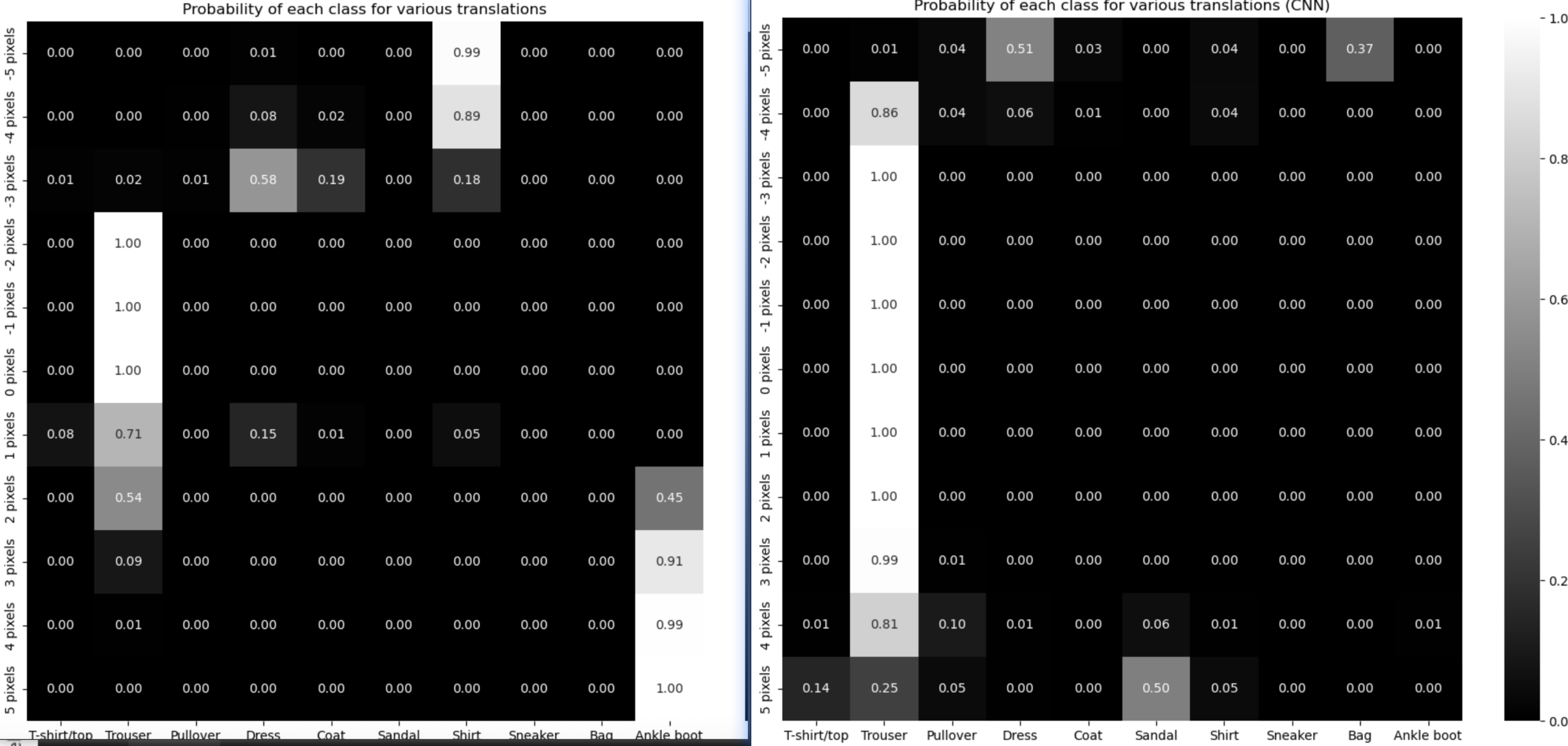
两次结果放到一起对比，发现卷积神经网络在像素平移之后仍然具有很好的识别性