


转自:http://www.db110.com/%E9%98%BF%E5%A7%86%E8%BE%BE%E5%B0%94%E5%AE%9A%E5%BE%8Bamdahls-law/
阿姆达尔定律是一个计算机科学界的经验法则,因IBM公司计算机架构师吉恩·阿姆达尔而得名。吉恩·阿姆达尔在1967年发表的论文中提出了这个重要定律。
阿姆达尔定律主要用于发现仅仅系统的部分得到改进,整体系统可以得到的最大期望改进。它经常用于并行计算领域,用来预测适用多个处理器时理论上的最大加速比。在我们的性能调优领域,我们利用此定律有助于我们解决或者缓解性能瓶颈问题。
阿姆达尔定律的模型阐释了我们现实生产中串行资源争用时候的现象。如下图模型,一个系统中,不可避免有一些资源必须串行访问,这限制了我们的加速比,即使我们增加了并发数(横轴),但取得效果并不理想,难以获得线性扩展能力(图中直线)。

以下介绍中、系统、算法、程序可以认为都是优化的对象,我不加以区分,它们都有串行的部分和可以并行的部分。
在并行计算中,使用多个处理器的程序的加速比受限制于程序串行部分的执行时间。例如,如果一个程序使用一个CPU核执行需要20小时,其中部分代码只能串行,需要执行1个小时,其他19小时的代码执行可以并行,那么,不考虑有多少CPU可用来并行执行程序,最小执行时间不会小于1小时(串行工作的部分),因此加速比被限制为最多20倍(20/1)。
加速比越高,证明优化效果越明显。
阿姆达尔定律可以用如下公式表示:
![]()
- s( n ) 固定负载下,理论上的加速比
- B 串行工作部分所占比例,取值0~1
- n 并行线程数、并行处理节点个数
以上公式说明:
加速比=没有改进前的算法耗时/改进后的算法耗时
如果我们假定算法没有改进之前,执行总时间是1(假定为1个单元)。那么改进后的算法,其时间应该是串行工作部分的耗时(B)加上并行部分的耗时(1-B)/n,由于并行部分可以在多个cpu核上执行,所以并行部分实际的执行时间是(1-B)/n
根据这个公式,如果并行线程数(我们可以理解为CPU处理器数量)趋于无穷,那么加速比与系统的串行工作部分的比例成反比,如果系统中有50%的代码串行执行,那么系统的最大加速比为2。也就是说,为了提高系统的速度,仅增加CPU处理器的数量不一定能起到有效的作用,需要提高系统内可并行化的模块比重,在此基础上合理增加并行处理器数量,才能以最小的投入得到最大的加速比。
对阿姆达尔定律做进一步说明。阿姆达尔这个模型 定义了固定负载下,某个算法的并行实现相对串行实现的加速比。例如,某个算法有12%的操作是可以并行执行的,而剩下的88%的操作不能并行,那么阿姆达尔定律声明,最大加速比是1(1-0.12)=1.136。如上公式n趋向于无穷大,那么加速比S=1/B=1/(1-0.12)。
再例如,对于某个算法,可以并行的比例是P,这部分并行的代码能够加速s倍(s可以理解是CPU核的个数,即新代码的执行时间为原来执行时间的1/s)。此算法30%的代码可以被并行加速,那么P等于0.3,这部分代码可以被加速2倍,s等于2。那么,使用阿姆达尔定律计算其整个算法的加速比:
![]()
以上公式和前一个公式类似,只是前一个公式的分母用串行比例B来表示。
再例如,某项任务,我们可以分解为4个步骤,P1、P2、P3、P4,执行耗时占总耗时百分比分别是11%、18%、23%、48%。我们对它进行优化,P1不能优化,P2可以加速5倍,P3可以加速20倍,P4可以加速1.6倍。那么改进后的执行时间是:
![]()
总的加速比是 1 / 0.4575 = 2.186 。我们可以看到,虽然有些部分加速比有20倍,5倍,但总的加速比并不高,略大于2,因为占时间比例最大的P4部分仅仅加速了1.6倍。
对于如下的图,我们可以观察到,加速比受限制于串行工作部分的比例,当95%的代码都可以进行并行优化时,理论的最大大加速比会更高,但最高不会超过20倍。

阿姆达尔定律也用于指导CPU的可扩展设计。CPU的发展有两个方向,更快的CPU或者更多的核。目前看来发展的重心偏向了CPU的核数,随着技术的不断发展,CPU的核数不断增加,目前我们的数据库服务器四核、六核已经比较常见,但有时我们会发现虽然拥有更多的核,当我们同时运行几个程序时,只有少数几个线程处于工作中,其它的并未做什么工作,实践当中,并行运行多个线程往往并不能显著提升性能,程序往往并不能有效的利用多核。在多核处理器中加速比是衡量并行程序性能的一个重要参数,能否有效降低串行计算部分的比例和降低交互开销决定了能否充分发挥多核的性能,其中的关键在于:合理划分任务、减少核间通信。
以计算机架构师吉恩·阿姆达尔的名字命名的定律,用于寻找仅对系统的一部分进行改进时整个系统预期得到的最大改进。换言之,该定律要讨论的是为什么增加某些东西并不总能带来能力的翻番。该定律可应用在计算机行业,比如研究CPU的核数与性能的关系;在高性能计算领域,该定律可以解释为什么增加节点并不能带来性能的线性改善。
阿姆达尔定律证明
Speedup(due to EnhanceMent E) = ExcuteTime(without E)/ExcuteTime(With E) = Performance(With E)/Performanc(Without E)

Suppose the enhancement E accelerates a fraction P of one task by a factor S and the remainder of the task unaffected then:

ExcuteTime(With E) = {(1-P) + P/S} * ExcuteTime(Without E);

Speedup(E) = 1/{(1-P)+P/S};
以上就是Amdahl's law证明。
Amdahl's law主要的用途是指出了在计算机体系结构设计过程中,某个部件的优化对整个结构的优化帮助是有上限的,这个极限就是当S→∞时,speedup(E) = 1/(1-P);也从另外一个方面说明了在体系结构的优化设计过程中,应该挑选对整体有重大影响的部件来进行优化,以得到更好的结果。
Amdahl's Law & Parallel Speedup
The theory of doing computational work in parallel has some fundamental laws that place limits on the benefits one can derive from parallelizing a computation (or really, any kind of work). To understand these laws, we have to first define the objective. In general, the goal in large scale computation is to get as much work done as possible in the shortest possible time within our budget. We ``win'' when we can do a big job in less time or a bigger job in the same time and not go broke doing so. The ``power'' of a computational system might thus be usefully defined to be the amount of computational work that can be done divided by the time it takes to do it, and we generally wish to optimize power per unit cost, or cost-benefit.
Physics and economics conspire to limit the raw power of individual single processor systems available to do any particular piece of work even when the dollar budget is effectively unlimited. The cost-benefit scaling of increasingly powerful single processor systems is generally nonlinear and very poor - one that is twice as fast might cost four times as much, yielding only half the cost-benefit, per dollar, of a cheaper but slower system. One way to increase the power of a computational system (for problems of the appropriate sort) past the economically feasible single processor limit is to apply more than one computational engine to the problem.
This is the motivation for beowulf design and construction; in many cases a beowulf may provide access to computational power that is available in a alternative single or multiple processor designs, but only at a far greater cost.
In a perfect world, a computational job that is split up among ![]() processors would
complete in
processors would
complete in ![]() time, leading to an
time, leading to an ![]() -fold increase in power. However, any given piece of
parallelized work to be done will contain parts of the work that must
be done serially, one task after another, by a single processor. This part does
not run any faster on a parallel collection of processors (and might
even run more slowly). Only the part that can be parallelized runs as much as
-fold increase in power. However, any given piece of
parallelized work to be done will contain parts of the work that must
be done serially, one task after another, by a single processor. This part does
not run any faster on a parallel collection of processors (and might
even run more slowly). Only the part that can be parallelized runs as much as
![]() -fold
faster.
-fold
faster.
The ``speedup'' of a parallel program is defined to be the ratio of the rate
at which work is done (the power) when a job is run on ![]() processors to the rate at which
it is done by just one. To simplify the discussion, we will now consider the
``computational work'' to be accomplished to be an arbitrary task (generally
speaking, the particular problem of greatest interest to the reader). We can
then define the speedup (increase in power as a function of
processors to the rate at which
it is done by just one. To simplify the discussion, we will now consider the
``computational work'' to be accomplished to be an arbitrary task (generally
speaking, the particular problem of greatest interest to the reader). We can
then define the speedup (increase in power as a function of ![]() ) in terms of the time
required to complete this particular fixed piece of work on 1 to
) in terms of the time
required to complete this particular fixed piece of work on 1 to ![]() processors.
processors.
Let ![]() be the time required to complete the task on
be the time required to complete the task on ![]() processors. The speedup
processors. The speedup ![]() is the
ratio
is the
ratio
| (1) |
In many cases the time ![]() has, as noted above, both a serial portion
has, as noted above, both a serial portion ![]() and a parallelizeable
portion
and a parallelizeable
portion ![]() . The serial time does not diminish when the parallel part is split
up. If one is "optimally" fortunate, the parallel time is decreased by a factor
of
. The serial time does not diminish when the parallel part is split
up. If one is "optimally" fortunate, the parallel time is decreased by a factor
of ![]() ). The
speedup one can expect is thus
). The
speedup one can expect is thus
| (2) |
This elegant expression is known as Amdahl's Law [Amdahl] and is usually expressed as an inequality.
This is in almost all cases the best speedup one can achieve by doing
work in parallel, so the real speed up ![]() is less than or equal to this quantity.
is less than or equal to this quantity.
Amdahl's Law immediately eliminates many, many tasks from consideration for parallelization. If the serial fraction of the code is not much smaller than the part that could be parallelized (if we rewrote it and were fortunate in being able to split it up among nodes to complete in less time than it otherwise would), we simply won't see much speedup no matter how many nodes or how fast our communications. Even so, Amdahl's law is still far too optimistic. It ignores the overhead incurred due to parallelizing the code. We must generalize it.
A fairer (and more detailed) description of parallel speedup includes at least two more times of interest:
![${\bf T_s}$]() The original single-processor serial time.
The original single-processor serial time.
![${\bf T_{is}}$]() The (average) additional serial time spent doing things like
interprocessor communications (IPCs), setup, and so forth in all parallelized
tasks. This time can depend on
The (average) additional serial time spent doing things like
interprocessor communications (IPCs), setup, and so forth in all parallelized
tasks. This time can depend on ![$N$]() in a variety of ways, but the simplest assumption is
that each system has to expend this much time, one after the other, so that the
total additional serial time is for example
in a variety of ways, but the simplest assumption is
that each system has to expend this much time, one after the other, so that the
total additional serial time is for example ![$N*T_{is}$]() .
.
![${\bf T_p}$]() The original single-processor parallelizeable time.
The original single-processor parallelizeable time.
![${\bf T_{ip}}$]() The (average) additional time spent by each processor doing
just the setup and work that it does in parallel. This may well include idle
time, which is often important enough to be accounted for separately.
The (average) additional time spent by each processor doing
just the setup and work that it does in parallel. This may well include idle
time, which is often important enough to be accounted for separately.
It is worth remarking that generally, the most important element that
contributes to ![]() is the time required for communication between the parallel subtasks.
This communication time is always there - even in the simplest parallel models
where identical jobs are farmed out and run in parallel on a cluster of
networked computers, the remote jobs must be begun and controlled with messages
passed over the network. In more complex jobs, partial results developed on each
CPU may have to be sent to all other CPUs in the beowulf for the calculation to
proceed, which can be very costly in scaled time. As we'll see below,
is the time required for communication between the parallel subtasks.
This communication time is always there - even in the simplest parallel models
where identical jobs are farmed out and run in parallel on a cluster of
networked computers, the remote jobs must be begun and controlled with messages
passed over the network. In more complex jobs, partial results developed on each
CPU may have to be sent to all other CPUs in the beowulf for the calculation to
proceed, which can be very costly in scaled time. As we'll see below,
![]() in
particular plays an extremely important role in determining the speedup scaling
of a given calculation. For this (excellent!) reason many beowulf designers and
programmers are obsessed with communications hardware and algorithms.
in
particular plays an extremely important role in determining the speedup scaling
of a given calculation. For this (excellent!) reason many beowulf designers and
programmers are obsessed with communications hardware and algorithms.
It is common to combine ![]() ,
, ![]() and
and ![]() into a single expression
into a single expression ![]() (the ``overhead time'') which
includes any complicated
(the ``overhead time'') which
includes any complicated ![]() -scaling of the IPC, setup, idle, and other times
associated with the overhead of running the calculation in parallel, as well as
the scaling of these quantities with respect to the ``size'' of the task being
accomplished. The description above (which we retain as it illustrates the
generic form of the relevant scalings) is still a simplified
description of the times - real life parallel tasks can be much more
complicated, although in many cases the description above is adequate.
-scaling of the IPC, setup, idle, and other times
associated with the overhead of running the calculation in parallel, as well as
the scaling of these quantities with respect to the ``size'' of the task being
accomplished. The description above (which we retain as it illustrates the
generic form of the relevant scalings) is still a simplified
description of the times - real life parallel tasks can be much more
complicated, although in many cases the description above is adequate.
Using these definitions and doing a bit of algebra, it is easy to show that
an improved (but still simple) estimate for the parallel speedup resulting from
splitting a particular job up between ![]() nodes (assuming one processor per node) is:
nodes (assuming one processor per node) is:
This expression will suffice to get at least a general feel for the scaling properties of a task that might be parallelized on a typical beowulf.
It is useful to plot the dimensionless ``real-world speedup'' (3) for various relative values of the times.
In all the figures below, ![]() = 10 (which sets our basic scale, if you like) and
= 10 (which sets our basic scale, if you like) and ![]() = 10, 100,
1000, 10000, 100000 (to show the systematic effects of parallelizing more and
more work compared to
= 10, 100,
1000, 10000, 100000 (to show the systematic effects of parallelizing more and
more work compared to ![]() ).
).
The primary determinant of beowulf scaling performance is the amount of
(serial) work that must be done to set up jobs on the nodes and then in
communications between the nodes, the time that is represented as ![]() . All figures have
. All figures have
![]() fixed; this parameter is rather boring as it effectively adds to
fixed; this parameter is rather boring as it effectively adds to ![]() and is often
very small.
and is often
very small.
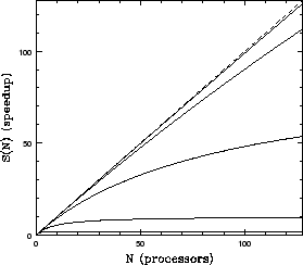
Figure 1 shows the kind of scaling one sees when communication times are
negligible compared to computation. This set of curves is roughly what one
expects from Amdahl's Law alone, which was derived with no consideration of IPC
overhead. Note that the dashed line in all figures is perfectly linear speedup,
which is never obtained over the entire range of ![]() although one can often come
close for small
although one can often come
close for small ![]() or large enough
or large enough ![]() .
.
In figure 2, we show a fairly typical curve for a ``real'' beowulf, with a
relatively small IPC overhead of ![]() . In this figure one can see the
advantage of cranking up the parallel fraction (
. In this figure one can see the
advantage of cranking up the parallel fraction (![]() relative to
relative to ![]() ) and can also see how
even a relatively small serial communications process on each node causes the
gain curves to peak well short of the saturation predicted by Amdahl's Law in
the first figure. Adding processors past this point costs one speedup.
Increasing
) and can also see how
even a relatively small serial communications process on each node causes the
gain curves to peak well short of the saturation predicted by Amdahl's Law in
the first figure. Adding processors past this point costs one speedup.
Increasing ![]() further (relative to everything else) causes the speedup curves to
peak earlier and at smaller values.
further (relative to everything else) causes the speedup curves to
peak earlier and at smaller values.
Finally, in figure 3 we continue to set ![]() , but this time with a
quadratic
, but this time with a
quadratic ![]() dependence
dependence ![]() of the serial IPC time. This might result if the
communications required between processors is long range (so every processor
must speak to every other processor) and is not efficiently managed by a
suitable algorithm. There are other ways to get nonlinear dependences of the
additional serial time on
of the serial IPC time. This might result if the
communications required between processors is long range (so every processor
must speak to every other processor) and is not efficiently managed by a
suitable algorithm. There are other ways to get nonlinear dependences of the
additional serial time on ![]() , and as this figure clearly shows they can have a
profound effect on the per-processor scaling of the speedup.
, and as this figure clearly shows they can have a
profound effect on the per-processor scaling of the speedup.
 |
As one can clearly see, unless the ratio of ![]() to
to ![]() is in the ballpark of 100,000 to
1 one cannot actually benefit from having 128 processors in a
``typical'' beowulf. At only 10,000 to 1, the speedup saturates at around 100
processors and then decreases. When the ratio is even smaller, the speedup peaks
with only a handful of nodes working on the problem. From this we learn some
important lessons. The most important one is that for many problems simply
adding processors to a beowulf design won't provide any additional speedup and
could even slow a calculation down unless one also scales up the
problem (increasing the
is in the ballpark of 100,000 to
1 one cannot actually benefit from having 128 processors in a
``typical'' beowulf. At only 10,000 to 1, the speedup saturates at around 100
processors and then decreases. When the ratio is even smaller, the speedup peaks
with only a handful of nodes working on the problem. From this we learn some
important lessons. The most important one is that for many problems simply
adding processors to a beowulf design won't provide any additional speedup and
could even slow a calculation down unless one also scales up the
problem (increasing the ![]() to
to ![]() ratio) as well.
ratio) as well.
The scaling of a given calculation has a significant impact on beowulf
engineering. Because of overhead, speedup is not a matter of just adding the
speed of however many nodes one applies to a given problem. For some problems it
is clearly advantageous to trade off the number of nodes one purchases
(for example in a problem with small ![]() and
and
![]() )
in order to purchase tenfold improved communications (and perhaps alter the
)
in order to purchase tenfold improved communications (and perhaps alter the ![]() ratio
to 1000).
ratio
to 1000).
The nonlinearities prevent one from developing any simple rules of thumb in
beowulf design. There are times when one obtains the greatest benefit by
selecting the fastest possible processors and network (which reduce both ![]() and
and ![]() in absolute
terms) instead of buying more nodes because we know that the rate equation above
will limit the parallel speedup we might ever hope to get even with the fastest
nodes. Paradoxically, there are other times that we can do better (get better
speedup scaling, at any rate) by buying slower processors (when we are
network bound, for example), as this can also increase
in absolute
terms) instead of buying more nodes because we know that the rate equation above
will limit the parallel speedup we might ever hope to get even with the fastest
nodes. Paradoxically, there are other times that we can do better (get better
speedup scaling, at any rate) by buying slower processors (when we are
network bound, for example), as this can also increase ![]() . In general,
one should be aware of the peaks that occur at the various scales and not
naively distribute small calculations (with small
. In general,
one should be aware of the peaks that occur at the various scales and not
naively distribute small calculations (with small ![]() ) over more processors than they
can use.
) over more processors than they
can use.
In summary, parallel performance depends primarily on certain relatively
simple parameters like ![]() ,
, ![]() and
and ![]() (although there may well be a devil in the details that
we've passed over). These parameters, in turn are at least partially under our
control in the form of programming decisions and hardware design decisions.
Unfortunately, they depend on many microscopic measures of system and network
performance that are inaccessible to many potential beowulf designers and users.
(although there may well be a devil in the details that
we've passed over). These parameters, in turn are at least partially under our
control in the form of programming decisions and hardware design decisions.
Unfortunately, they depend on many microscopic measures of system and network
performance that are inaccessible to many potential beowulf designers and users.
![]() clearly
should depend on the ``speed'' of a node, but the single node speed itself may
depend nonlinearly on the speed of the processor, the size and
structure of the caches, the operating system, and more.
clearly
should depend on the ``speed'' of a node, but the single node speed itself may
depend nonlinearly on the speed of the processor, the size and
structure of the caches, the operating system, and more.
Because of the nonlinear complexity, there is no way to a priori estimate expected performance on the basis of any simple measure. There is still considerable benefit to be derived from having in hand a set of quantitative measures of ``microscopic'' system performance and gradually coming to understand how one's program depends on the potential bottlenecks they reveal. The remainder of this paper is dedicated to reviewing the results of applying a suite of microbenchmark tools to a pair of nodes to provide a quantitative basis for further beowulf hardware and software engineering.
Robert G. Brown 2000-08-28

 浙公网安备 33010602011771号