
泰坦尼克号生存预测——哪些群体的乘客在泰坦尼克号沉船事故中更容易幸存下来
一、选题背景
"泰坦尼克号"在与冰山相撞后沉没。船上的每个人都没有足够的救生艇,导致2224名乘客和船员中有1502人死亡。虽然能否存活是要靠有一些运气因素,但似乎有些比其他群体更有可能生存下来。本课题探究不同群体的乘客,例如:社会阶级(贵族和平民);经济因素;年龄段;性别;所处的船仓级别;在船上的头衔都会影响存活率。是什么样的群体更容易在这次灾难中存活。
二、机器学习案例和设计方案
1.本选题的采用的训练集与测试集来源于Kaggle官网 Kaggle: Your Home for Data Science
(说明:test.csv 是用于预测乘客是否能存活下来的测试集)
2.本课题采用的数学模型:(1)Gaussian Naive Bayes
(2) Logistic Regression
(3) Random Forest
(4)KNN or k-Nearest Neighbors
(学习参考来源于: (10条消息) python实现 Gaussian naive bayes高斯朴素贝叶斯_WYXHAHAHA123的博客-CSDN博客
(10条消息) GBDT之GradientBoostingClassifier源码分析_Mr·董จุ๊บ的博客-CSDN博客_gradientboostingclassifier)
(10条消息) 一、K -近邻算法(KNN:k-Nearest Neighbors)_沈波的专栏-CSDN博客
(10条消息) 随机森林算法及其实现(Random Forest)_AAA小肥杨的博客-CSDN博客_随机森林
特此感谢,对我课题研究有很大帮助
3. 遇到的难题: 精确度普遍不高,本人现阶段所能使用的方法就是优化数据,更换数学模型。
三、机器学习实现步骤
(1)导入必要的库,数据集
首先导入所需要的库。
1 #首先导入所需要的库
2 import numpy as np
3 import pandas as pd
4 import matplotlib.pyplot as plt
5 import seaborn as sns
6 %matplotlib inline
7 #忽略无关紧要的警告
8 import warnings
9 warnings.filterwarnings('ignore')
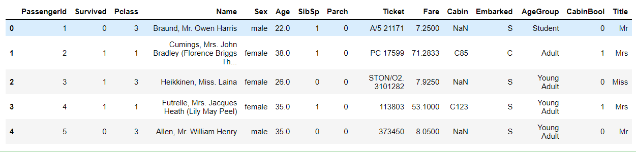
导入训练集,测试集,并查看其内容。
1 #导入训练集和测试集CSV文件
2 train = pd.read_csv("D:/Titanic/train.csv")
3 test = pd.read_csv("D:/Titanic/test.csv")
4 #查看训练集的内容
5 train.describe(include="all")
out:

(2)数据分析
获取数据的特征名称,并随机选取5组数据了解其变量
1 #获取训练集的索引列名
2 print(train.columns)
3 #随机选取5组数据
4 train.sample(5)
out:
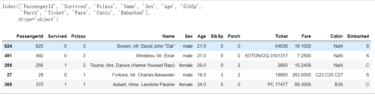
注释: Pcalss:船票舱位 SibSp:同乘坐这艘船的兄弟姐妹或配偶的人数
Cabin:客舱号 Embarked:登船港口(S=Southampton,C = Cherbourg, Q = Queenstown)
通过上述的操作,大致了解训练集数据,并有以下的结论,针对其进一步对数据进行处理。
我们的训练集中总共有891名乘客。
(1)Age特征缺少约20%的值 。缺少较少,我们应尽可能的为此填充数据.
(2) Cabin特征缺少其值的大约80%。由于缺少这么,因此很难填充缺少的值。我会从数据集中删除这些值。
#进一步查看缺失值的数据的个数
print(pd.isnull(train).sum())
out:

本人有以下猜想:
(1)女性相比男性会有更多存活率。
(2)独自坐船的人或只有一个兄弟姐妹的乘客更有可能被获救。
(3)小孩相比成年人更有可能被获救。
(4)更高级的船舱的人更有可能被获救。
(3)数据可视化
接下来运用数据可视化所学的知识对猜想进一步验证
Sex
#绘制一个关于 ”性别 “的条形图
sns.barplot(x="Sex", y="Survived", data=train)
#给出男性跟女性的存活率
print("Percentage of females who survived:", train["Survived"][train["Sex"] == 'female'].value_counts(normalize = True)[1]*100)
print("Percentage of males who survived:", train["Survived"][train["Sex"] == 'male'].value_counts(normalize = True)[1]*100)
out:
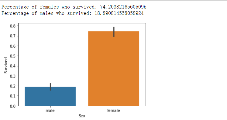
(根据统计图,女性比男性有更高的存活率,符合猜想)
Pclass(船票舱位)
#绘制船票舱位与存活率的关系条形图
sns.barplot(x="Pclass", y="Survived", data=train)
#给出相应的百分比
print("Percentage of Pclass = 1 who survived:", train["Survived"][train["Pclass"] == 1].value_counts(normalize = True)[1]*100)

print("Percentage of Pclass = 2 who survived:", train["Survived"][train["Pclass"] == 2].value_counts(normalize = True)[1]*100)

print("Percentage of Pclass = 3 who survived:", train["Survived"][train["Pclass"] == 3].value_counts(normalize = True)[1]*100)
out:

(符合猜想)
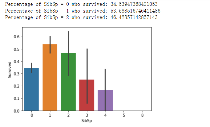
Sibsp(同行的兄弟姐妹人数)
1 #绘制Sibsp和存活率的关系直方图
2 sns.barplot(x="SibSp", y="Survived", data=train)
3 #给出相应的百分占比
4 print("Percentage of SibSp = 0 who survived:", train["Survived"][train["SibSp"] == 0].value_counts(normalize = True)[1]*100)
5 print("Percentage of SibSp = 1 who survived:", train["Survived"][train["SibSp"] == 1].value_counts(normalize = True)[1]*100)
6 print("Percentage of SibSp = 2 who survived:", train["Survived"][train["SibSp"] == 2].value_counts(normalize = True)[1]*100)
out:
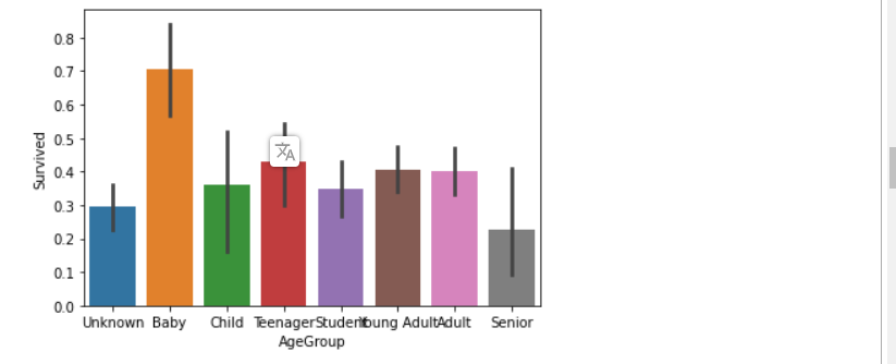
年龄段
#把年龄进行分类
train["Age"] = train["Age"].fillna(-0.5)
test["Age"] = test["Age"].fillna(-0.5)
bins = [-1, 0, 5, 12, 18, 24, 35, 60, np.inf]
labels = ['Unknown', 'Baby', 'Child', 'Teenager', 'Student', 'Young Adult', 'Adult', 'Senior']
train['AgeGroup'] = pd.cut(train["Age"], bins, labels = labels)
test['AgeGroup'] = pd.cut(test["Age"], bins, labels = labels)
#绘制关系直方图
sns.barplot(x="AgeGroup", y="Survived", data=train)
plt.show()
out:
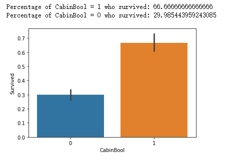
船舱号(Cabin)
 1 train["CabinBool"] = (train["Cabin"].notnull().astype('int'))
 2 test["CabinBool"] = (test["Cabin"].notnull().astype('int'))
 3
 4 #calculate percentages of CabinBool vs. survived
 5 print("Percentage of CabinBool = 1 who survived:", train["Survived"][train["CabinBool"] == 1].value_counts(normalize = True)[1]*100)
 6
 7 print("Percentage of CabinBool = 0 who survived:", train["Survived"][train["CabinBool"] == 0].value_counts(normalize = True)[1]*100)
 8 #绘制一个CabinBool与Survived 关系条形图
 9 sns.barplot(x="CabinBool", y="Survived", data=train)
10 plt.show()
out:
(4)数据清理
下一步我打算清理数据以便处理缺失值和不必要的信息
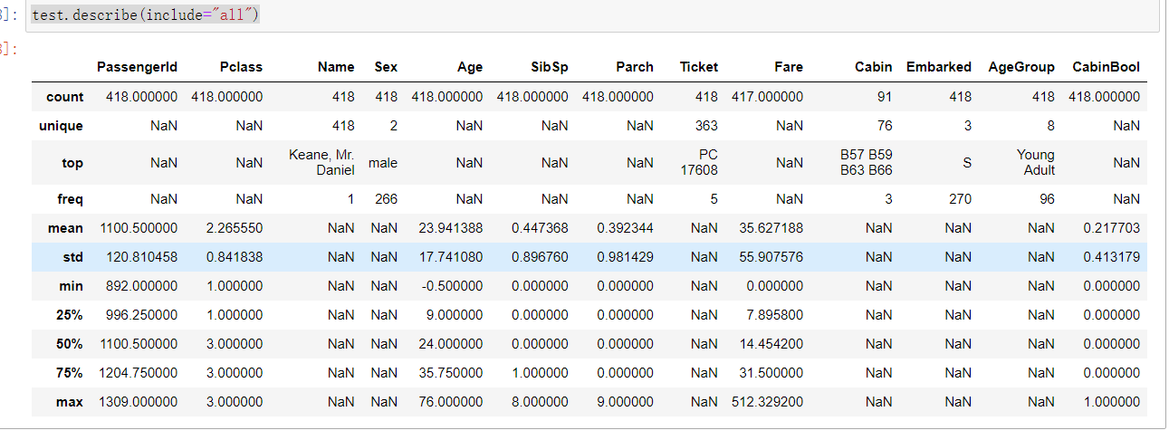
首先先浏览一下测试集
test.describe(include="all")
out:
删除一些不必要的数据
(1)Cabin
#对于存活率的预测没什么有用的信息,剔除它
train = train.drop(['Cabin'], axis = 1)
test = test.drop(['Cabin'], axis = 1)
(2)Ticket
#票证,没有什么有用的信息
train = train.drop(['Ticket'], axis = 1)
test = test.drop(['Ticket'], axis = 1)
增添一些缺失值
(1)Embarked
(找出乘客登船最多的港口,用那个港口的名称替换缺失值)
#找出最多乘客登船的港口
print("Number of people embarking in Southampton (S):")
southampton = train[train["Embarked"] == "S"].shape[0]
print(southampton)
print("Number of people embarking in Cherbourg (C):")
cherbourg = train[train["Embarked"] == "C"].shape[0]
print(cherbourg)
print("Number of people embarking in Queenstown (Q):")
queenstown = train[train["Embarked"] == "Q"].shape[0]
print(queenstown)
上述得出S港最多人登船,用此替换缺失值。
#用S港替换缺失值
train = train.fillna({"Embarked": "S"})
(2)Age
本课题难点之一:年龄缺失值很多,用刚才找出出现最多的填充明显不符合逻辑
所以这边用了一个预测年龄的方法填充缺少值
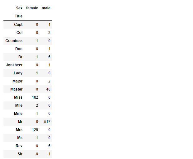
#这边创建了两个数据集的组合组
combine = [train, test]
#从训练集和测试集提取一个适当的标题
for dataset in combine:
    dataset['Title'] = dataset.Name.str.extract(' ([A-Za-z]+)\.', expand=False)
pd.crosstab(train['Title'], train['Sex'])
out:
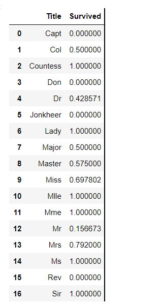
 1 #用更常见的名称替换各种标题
 2 for dataset in combine:
 3     dataset['Title'] = dataset['Title'].replace(['Lady', 'Capt', 'Col',
 4     'Don', 'Dr', 'Major', 'Rev', 'Jonkheer', 'Dona'], 'Rare')
 5
 6     dataset['Title'] = dataset['Title'].replace(['Countess', 'Lady', 'Sir'], 'Royal')
 7     dataset['Title'] = dataset['Title'].replace('Mlle', 'Miss')
 8     dataset['Title'] = dataset['Title'].replace('Ms', 'Miss')
 9     dataset['Title'] = dataset['Title'].replace('Mme', 'Mrs')
10
11 train[['Title', 'Survived']].groupby(['Title'], as_index=False).mean()
out:
1 #将每个标题组映射到一个数值
2 title_mapping = {"Mr": 1, "Miss": 2, "Mrs": 3, "Master": 4, "Royal": 5, "Rare": 6}
3 for dataset in combine:
4     dataset['Title'] = dataset['Title'].map(title_mapping)
5     dataset['Title'] = dataset['Title'].fillna(0)
6
7 train.head()
out:
接下来,我们将尝试从标题的最常见年龄预测缺少的年龄值。
#用每个标题的模式年龄组填充缺少的年龄
mr_age = train[train["Title"] == 1]["AgeGroup"].mode() #Young Adult
miss_age = train[train["Title"] == 2]["AgeGroup"].mode() #Student
mrs_age = train[train["Title"] == 3]["AgeGroup"].mode() #Adult
master_age = train[train["Title"] == 4]["AgeGroup"].mode() #Baby
royal_age = train[train["Title"] == 5]["AgeGroup"].mode() #Adult
rare_age = train[train["Title"] == 6]["AgeGroup"].mode() #Adult

age_title_mapping = {1: "Young Adult", 2: "Student", 3: "Adult", 4: "Baby", 5: "Adult", 6: "Adult"}
for x in range(len(train["AgeGroup"])):
    if train["AgeGroup"][x] == "Unknown":
        train["AgeGroup"][x] = age_title_mapping[train["Title"][x]]

for x in range(len(test["AgeGroup"])):
    if test["AgeGroup"][x] == "Unknown":
        test["AgeGroup"][x] = age_title_mapping[test["Title"][x]]
现在已经以一种较准确的方式填充了缺失值,接下来把把每一个年龄组映射到每一个数值。
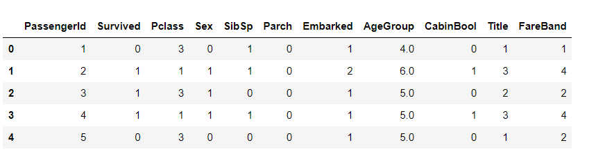
1 #将每个年龄的值映射到相应的地方
2 age_mapping = {'Baby': 1, 'Child': 2, 'Teenager': 3, 'Student': 4, 'Young Adult': 5, 'Adult': 6, 'Senior': 7}
3 train['AgeGroup'] = train['AgeGroup'].map(age_mapping)
4 test['AgeGroup'] = test['AgeGroup'].map(age_mapping)
5
6 train.head()
现在已经提取了标题,可以删除“姓名”这一特征的列了
1 #删除“Name”一列
2 train = train.drop(['Name'], axis = 1)
3 test = test.drop(['Name'], axis = 1)
1 #将每个性别值映射到一个数值
2 sex_mapping = {"male": 0, "female": 1}
3 train['Sex'] = train['Sex'].map(sex_mapping)
4 test['Sex'] = test['Sex'].map(sex_mapping)
5
6 train.head()
out:
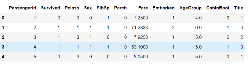
1 #将登港口每个值映射为相应数值
2 embarked_mapping = {"S": 1, "C": 2, "Q": 3}
3 train['Embarked'] = train['Embarked'].map(embarked_mapping)
4 test['Embarked'] = test['Embarked'].map(embarked_mapping)
5 train.head()
out:
接下来依照Pclass的等级把Fare(票价)进行分组,并填充缺失值。
1 #根据Pclass的平均票价,在测试集中填写缺失的票价值
2 for x in range(len(test["Fare"])):
3     if pd.isnull(test["Fare"][x]):
4         pclass = test["Pclass"][x] #Pclass = 3
5         test["Fare"][x] = round(train[train["Pclass"] == pclass]["Fare"].mean(), 4)
6 #将票价的值映射为一组数值
7 train['FareBand'] = pd.qcut(train['Fare'], 4, labels = [1, 2, 3, 4])
8 test['FareBand'] = pd.qcut(test['Fare'], 4, labels = [1, 2, 3, 4])
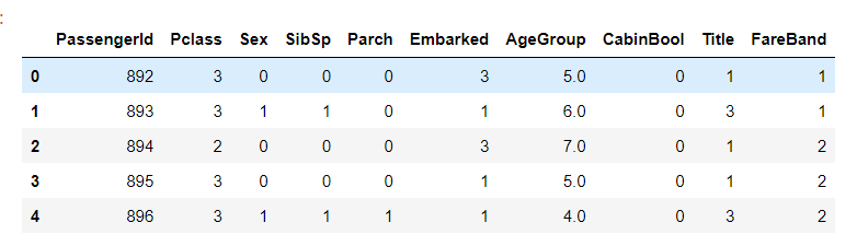
#查看现在训练集的数据
train.head()
out:

#查看一下现在测试集的数据
test.head()
out:
(5)模型训练
数据处理做完了,现在就来选择合适的模型。能力有限,只 用了四种模型。
1 #我们将使用部分训练数据(本例中为22%)来测试不同模型的准确性。
2 from sklearn.model_selection import train_test_split
3 predictors = train.drop(['Survived', 'PassengerId'], axis=1)
4 target = train["Survived"]
5 x_train, x_val, y_train, y_val = train_test_split(predictors, target, test_size = 0.22, random_state = 0)
对于每个模型,我只用80%的训练数据拟合,预测20%的训练数据,并检查准确性。
1 # Gaussian Naive Bayes
2 from sklearn.naive_bayes import GaussianNB
3 from sklearn.metrics import accuracy_score
4
5 gaussian = GaussianNB()
6 gaussian.fit(x_train, y_train)
7 y_pred = gaussian.predict(x_val)
8 acc_gaussian = round(accuracy_score(y_pred, y_val) * 100, 2)
9 print(acc_gaussian)
out:78.68
1 # Logistic Regression
2 from sklearn.linear_model import LogisticRegression
3
4 logreg = LogisticRegression()
5 logreg.fit(x_train, y_train)
6 y_pred = logreg.predict(x_val)
7 acc_logreg = round(accuracy_score(y_pred, y_val) * 100, 2)
8 print(acc_logreg)
out:79.70
1 # KNN or k-Nearest Neighbors
2 from sklearn.neighbors import KNeighborsClassifier
3
4 knn = KNeighborsClassifier()
5 knn.fit(x_train, y_train)
6 y_pred = knn.predict(x_val)
7 acc_knn = round(accuracy_score(y_pred, y_val) * 100, 2)
8 print(acc_knn)
out:77.66
1 # Random Forest
2 from sklearn.ensemble import RandomForestClassifier
3
4 randomforest = RandomForestClassifier()
5 randomforest.fit(x_train, y_train)
6 y_pred = randomforest.predict(x_val)
7 acc_randomforest = round(accuracy_score(y_pred, y_val) * 100, 2)
8 print(acc_randomforest)
out:85.79
接下来我们创建一个DataFrame来直观比较各个模型
1 models = pd.DataFrame({
2     'Model': [ 'KNN', 'Logistic Regression',
3               'Random Forest', 'Naive Bayes'],
4     'Score': [ acc_knn, acc_logreg,
5               acc_randomforest, acc_gaussian]})
6 models.sort_values(by='Score', ascending=False)
out:
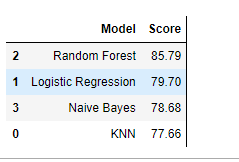
最终我选择 Random Forest 模型作为测试的结果。
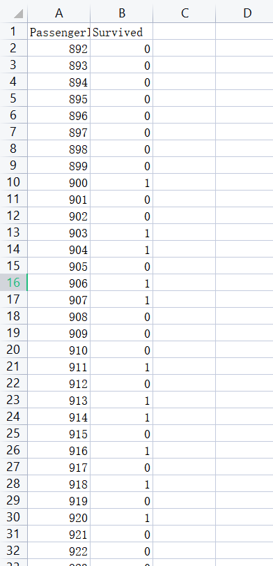
接下来生成一份测试结果的CSV文件
#将ids设置为PassengerId并预测生存率
ids = test['PassengerId']
predictions = randomforest.predict(test.drop('PassengerId', axis=1))

#生成一份测试结果CSV文件
output = pd.DataFrame({ 'PassengerId' : ids, 'Survived': predictions })
output.to_csv('测试结果.csv', index=False)
附上文件的一小部分截图
四:总结
1.结论:
要想提高训练精度,首先要对数据进行更规范,更准确的处理。本课题采用的训练集,包含许多缺失值和没有作用的信息。笔者在最开始,并没有对训练集数据进行优化处理,导致最后模型的精确度都特别低。
2.个人收获:
(1) 阅读了多篇关于机器学习的文章,对几个基础的训练模型有初步理解。
(2) 同时也对数据可视化的相关知识做了再复习。
3.个人反思(不足):
(1)对数据处理方面,只是简单的删除,填充,更换的方法,且占用的篇幅过长(本课题是对于机器学习,但有很大部分在整理数据和做数据可视化),最后对于模型的训练,也只是做了输出精确度,并没有更多的操作。
(2)需要对相关知识再做更深入的研究,了解更多提高精确度的方法。
(最后感谢Kaggle官网提供的数据集提高以及CSDN博主提供的资料与解答)
完整代码:
  1  #首先导入所需要的库
  2 import numpy as np
  3 import pandas as pd
  4 import matplotlib.pyplot as plt
  5 import seaborn as sns
  6 %matplotlib inline
  7 #忽略无关紧要的警告
  8 import warnings
  9 warnings.filterwarnings('ignore')
 10
 11 #导入训练集和测试集CSV文件
 12 train = pd.read_csv("D:/Titanic/train.csv")
 13 test = pd.read_csv("D:/Titanic/test.csv")
 14
 15 #查看训练集的内容
 16 train.describe(include="all")
 17
 18 #获取训练集的索引列名
 19 print(train.columns)
 20
 21 #随机选取5组数据
 22 train.sample(5)
 23
 24 #进一步查看缺失值的数据的个数
 25 print(pd.isnull(train).sum())
 26
 27 #绘制一个关于 ”性别 “的条形图
 28 sns.barplot(x="Sex", y="Survived", data=train)
 29
 30 #给出男性跟女性的存活率
 31 print("Percentage of females who survived:", train["Survived"][train["Sex"] == 'female'].value_counts(normalize = True)[1]*100)
 32 print("Percentage of males who survived:", train["Survived"][train["Sex"] == 'male'].value_counts(normalize = True)[1]*100)
 33
 34 #绘制船票舱位与存活率的关系条形图
 35 sns.barplot(x="Pclass", y="Survived", data=train)
 36
 37 #给出相应的百分比
 38 print("Percentage of Pclass = 1 who survived:", train["Survived"][train["Pclass"] == 1].value_counts(normalize = True)[1]*100)
 39
 40 print("Percentage of Pclass = 2 who survived:", train["Survived"][train["Pclass"] == 2].value_counts(normalize = True)[1]*100)
 41
 42 print("Percentage of Pclass = 3 who survived:", train["Survived"][train["Pclass"] == 3].value_counts(normalize = True)[1]*100)
 43
 44 #绘制Sibsp和存活率的关系直方图
 45 sns.barplot(x="SibSp", y="Survived", data=train)
 46
 47 #给出相应的百分占比
 48 print("Percentage of SibSp = 0 who survived:", train["Survived"][train["SibSp"] == 0].value_counts(normalize = True)[1]*100)
 49
 50 print("Percentage of SibSp = 1 who survived:", train["Survived"][train["SibSp"] == 1].value_counts(normalize = True)[1]*100)
 51
 52 print("Percentage of SibSp = 2 who survived:", train["Survived"][train["SibSp"] == 2].value_counts(normalize = True)[1]*100)
 53
 54 #把年龄进行分类
 55 train["Age"] = train["Age"].fillna(-0.5)
 56 test["Age"] = test["Age"].fillna(-0.5)
 57 bins = [-1, 0, 5, 12, 18, 24, 35, 60, np.inf]
 58 labels = ['Unknown', 'Baby', 'Child', 'Teenager', 'Student', 'Young Adult', 'Adult', 'Senior']
 59 train['AgeGroup'] = pd.cut(train["Age"], bins, labels = labels)
 60 test['AgeGroup'] = pd.cut(test["Age"], bins, labels = labels)
 61
 62 #绘制关系直方图
 63 sns.barplot(x="AgeGroup", y="Survived", data=train)
 64 plt.show()
 65 test.describe(include="all")
 66
 67 #对于存活率的预测没什么有用的信息,剔除它
 68 train = train.drop(['Cabin'], axis = 1)
 69 test = test.drop(['Cabin'], axis = 1)
 70
 71 #票证,没有什么有用的信息
 72 train = train.drop(['Ticket'], axis = 1)
 73 test = test.drop(['Ticket'], axis = 1)
 74
 75 #找出最多乘客登船的港口
 76 print("Number of people embarking in Southampton (S):")
 77 southampton = train[train["Embarked"] == "S"].shape[0]
 78 print(southampton)
 79
 80 print("Number of people embarking in Cherbourg (C):")
 81 cherbourg = train[train["Embarked"] == "C"].shape[0]
 82 print(cherbourg)
 83
 84 print("Number of people embarking in Queenstown (Q):")
 85 queenstown = train[train["Embarked"] == "Q"].shape[0]
 86 print(queenstown)
 87
 88 #用S港替换缺失值
 89 train = train.fillna({"Embarked": "S"})
 90
 91 #这边创建了两个数据集的组合组
 92 combine = [train, test]
 93
 94 #从训练集和测试集提取一个适当的标题
 95 for dataset in combine:
 96     dataset['Title'] = dataset.Name.str.extract(' ([A-Za-z]+)\.', expand=False)
 97 pd.crosstab(train['Title'], train['Sex'])
 98
 99 #用更常见的名称替换各种标题
100 for dataset in combine:
101     dataset['Title'] = dataset['Title'].replace(['Lady', 'Capt', 'Col',
102     'Don', 'Dr', 'Major', 'Rev', 'Jonkheer', 'Dona'], 'Rare')
103
104     dataset['Title'] = dataset['Title'].replace(['Countess', 'Lady', 'Sir'], 'Royal')
105
106     dataset['Title'] = dataset['Title'].replace('Mlle', 'Miss')
107
108     dataset['Title'] = dataset['Title'].replace('Ms', 'Miss')
109
110     dataset['Title'] = dataset['Title'].replace('Mme', 'Mrs')
111
112 train[['Title', 'Survived']].groupby(['Title'], as_index=False).mean()
113 train[['Title', 'Survived']].groupby(['Title'], as_index=False).mean()
114
115 #将每个标题组映射到一个数值
116 title_mapping = {"Mr": 1, "Miss": 2, "Mrs": 3, "Master": 4, "Royal": 5, "Rare": 6}
117 for dataset in combine:
118     dataset['Title'] = dataset['Title'].map(title_mapping)
119     dataset['Title'] = dataset['Title'].fillna(0)
120
121 train.head()
122
123 #用每个标题的模式年龄组填充缺少的年龄
124 mr_age = train[train["Title"] == 1]["AgeGroup"].mode() #Young Adult
125
126 miss_age = train[train["Title"] == 2]["AgeGroup"].mode() #Student
127
128 mrs_age = train[train["Title"] == 3]["AgeGroup"].mode() #Adult
129
130 master_age = train[train["Title"] == 4]["AgeGroup"].mode() #Baby
131
132 royal_age = train[train["Title"] == 5]["AgeGroup"].mode() #Adult
133
134 rare_age = train[train["Title"] == 6]["AgeGroup"].mode() #Adult
135 age_title_mapping = {1: "Young Adult", 2: "Student", 3: "Adult", 4: "Baby", 5: "Adult", 6: "Adult"}
136 for x in range(len(train["AgeGroup"])):
137     if train["AgeGroup"][x] == "Unknown":
138         train["AgeGroup"][x] = age_title_mapping[train["Title"][x]]
139
140 for x in range(len(test["AgeGroup"])):
141     if test["AgeGroup"][x] == "Unknown":
142         test["AgeGroup"][x] = age_title_mapping[test["Title"][x]]
143
144 #将每个年龄的值映射到相应的地方
145 age_mapping = {'Baby': 1, 'Child': 2, 'Teenager': 3, 'Student': 4, 'Young Adult': 5, 'Adult': 6, 'Senior': 7}
146 train['AgeGroup'] = train['AgeGroup'].map(age_mapping)
147 test['AgeGroup'] = test['AgeGroup'].map(age_mapping)
148
149 train.head()
150 #删除“Name”一列
151 train = train.drop(['Name'], axis = 1)
152 test = test.drop(['Name'], axis = 1)
153
154 #将每个性别值映射到一个数值
155 sex_mapping = {"male": 0, "female": 1}
156 train['Sex'] = train['Sex'].map(sex_mapping)
157 test['Sex'] = test['Sex'].map(sex_mapping)
158
159 train.head()
160 #将登港口每个值映射为相应数值
161 embarked_mapping = {"S": 1, "C": 2, "Q": 3}
162 train['Embarked'] = train['Embarked'].map(embarked_mapping)
163 test['Embarked'] = test['Embarked'].map(embarked_mapping)
164 train.head()
165
166 #根据Pclass的平均票价,在测试集中填写缺失的票价值
167 for x in range(len(test["Fare"])):
168      if pd.isnull(test["Fare"][x]):
169         pclass = test["Pclass"][x] #Pclass = 3
170         test["Fare"][x] = round(train[train["Pclass"] == pclass]["Fare"].mean(), 4)
171
172 #将票价的值映射为一组数值
173 train['FareBand'] = pd.qcut(train['Fare'], 4, labels = [1, 2, 3, 4])
174 test['FareBand'] = pd.qcut(test['Fare'], 4, labels = [1, 2, 3, 4])
175
176 #查看现在训练集的数据
177 train.head()
178
179 #查看一下现在测试集的数据
180 test.head()
181
182 #我们将使用部分训练数据(本例中为22%)来测试不同模型的准确性。
183 from sklearn.model_selection import train_test_split
184 predictors = train.drop(['Survived', 'PassengerId'], axis=1)
185 target = train["Survived"]
186 x_train, x_val, y_train, y_val = train_test_split(predictors, target, test_size = 0.22, random_state = 0)
187
188
189
190 # Gaussian Naive Bayes
191 from sklearn.naive_bayes import GaussianNB
192 from sklearn.metrics import accuracy_score
193
194 gaussian = GaussianNB()
195 gaussian.fit(x_train, y_train)
196 y_pred = gaussian.predict(x_val)
197 acc_gaussian = round(accuracy_score(y_pred, y_val) * 100, 2)
198 print(acc_gaussian)
199
200
201
202 # Logistic Regression
203 from sklearn.linear_model import LogisticRegression
204
205 logreg = LogisticRegression()
206 logreg.fit(x_train, y_train)
207 y_pred = logreg.predict(x_val)
208 acc_logreg = round(accuracy_score(y_pred, y_val) * 100, 2)
209 print(acc_logreg)
210
211
212
213 # KNN or k-Nearest Neighbors
214 from sklearn.neighbors import KNeighborsClassifier
215
216 knn = KNeighborsClassifier()
217 knn.fit(x_train, y_train)
218 y_pred = knn.predict(x_val)
219 acc_knn = round(accuracy_score(y_pred, y_val) * 100, 2)
220 print(acc_knn)
221
222
223
224 # Random Forest
225 from sklearn.ensemble import RandomForestClassifier
226
227 randomforest = RandomForestClassifier()
228 randomforest.fit(x_train, y_train)
229 y_pred = randomforest.predict(x_val)
230 acc_randomforest = round(accuracy_score(y_pred, y_val) * 100, 2)
231 print(acc_randomforest)
232
233
234 #列出每个模型的得出的acc
235 models = pd.DataFrame({
236      'Model': [ 'KNN', 'Logistic Regression',
237                'Random Forest', 'Naive Bayes'],
238      'Score': [ acc_knn, acc_logreg,
239               acc_randomforest, acc_gaussian]})
240  models.sort_values(by='Score', ascending=False)
241
242 #将ids设置为PassengerId并预测生存率
243 ids = test['PassengerId']
244 predictions = randomforest.predict(test.drop('PassengerId', axis=1))
245
246 #生成一份测试结果CSV文件
247 output = pd.DataFrame({ 'PassengerId' : ids, 'Survived': predictions })
248 output.to_csv('测试结果.csv', index=False)

 浙公网安备 33010602011771号