

一、选题背景
人脸识别技术是模式识别和计算机视觉领域最富挑战性的研究课题之一,也是近年来的研究热点。蔡徐坤作为新一代偶像,引人注目,外号鸡哥。真假kunkun识别就是向计算机输入坤坤或着鸡的图像,经过某种方法或运算,得出其结果。识别真假kunkun也受到了广泛地关注。这种识别对人眼来说很简单,但对计算机却并不是一件容易的事情。
二、机器学习案例设计方案
从网站中下载相关的数据集,对数据集进行整理,在python的环境中,给数据集中的文件进行划分,对数据进行预处理,利用keras,构建神经网络,训练模型,导入图片测试模型。
数据来源:kaggle,网址:The Kun Dataset (小黑子图库) | Kaggle 数据集包含2000多个jpg文件,其中1000+个是蔡徐坤照片,1000+个是鸡和鸡肉照片。
三、机器学习的实验步骤
1.下载数据集
2.导入需要用到的库
import os
import random
from shutil import copy
from matplotlib import pyplot as plt
from keras import optimizers
from keras import models
from keras import layers
from keras.preprocessing.image import ImageDataGenerator
from keras.models import load_model
from PIL import Image
3.数据集划分,由总的数据集生成分别生成训练集,测试集和验证集
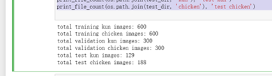
import os
from shutil import copy

# 定义路径和文件夹名
base_dir = r'D:\python'
train_dir = os.path.join(base_dir, 'train')
validation_dir = os.path.join(base_dir, 'validation')
test_dir = os.path.join(base_dir, 'test')

kun_train_dir = os.path.join(train_dir, 'kun')
kun_validation_dir = os.path.join(validation_dir, 'kun')
kun_test_dir = os.path.join(test_dir, 'kun')

chicken_train_dir = os.path.join(train_dir, 'chicken')
chicken_validation_dir = os.path.join(validation_dir, 'chicken')
chicken_test_dir = os.path.join(test_dir, 'chicken')

# 创建目录
dir_list = [kun_train_dir, kun_validation_dir, kun_test_dir,
            chicken_train_dir, chicken_validation_dir, chicken_test_dir]

for dir_child in dir_list:
    os.makedirs(dir_child, exist_ok=True)

# 复制文件到不同目录
def copy_files(source_path, destination_path, start_index, end_index):
    for i in range(start_index, end_index):
        child_path = os.path.join(source_path, os.listdir(source_path)[i])
        copy(child_path, destination_path)

# 复制kun图片
kun_path = r'D:\zwc\ikun\坤坤\坤坤'
kun_path_list = os.listdir(kun_path)

copy_files(kun_path, kun_train_dir, 0, 600)
copy_files(kun_path, kun_validation_dir, 600, 900)
copy_files(kun_path, kun_test_dir, 900, len(kun_path_list))

# 复制chicken图片
chicken_path = r'D:\zwc\ikun\只因\只因'
chicken_path_list = os.listdir(chicken_path)

copy_files(chicken_path, chicken_train_dir, 0, 600)
copy_files(chicken_path, chicken_validation_dir, 600, 900)
copy_files(chicken_path, chicken_test_dir, 900, len(chicken_path_list))

# 输出文件数量
def print_file_count(path, label):
    print('total', label, 'images:', len(os.listdir(path)))

print_file_count(os.path.join(train_dir, 'kun'), 'training kun')
print_file_count(os.path.join(train_dir, 'chicken'), 'training chicken')

print_file_count(os.path.join(validation_dir, 'kun'), 'validation kun')
print_file_count(os.path.join(validation_dir, 'chicken'), 'validation chicken')

print_file_count(os.path.join(test_dir, 'kun'), 'test kun')
print_file_count(os.path.join(test_dir, 'chicken'), 'test chicken')
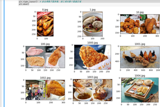
4.查看图像以及对应标签
# 查看图像以及对应的标签
fit, ax = plt.subplots(nrows=3, ncols=3, figsize=(10, 7))
# 查看图像的根路径
test_view_path = r'D:\python\test\chicken'
# 获取 test_view_path 下的文件夹列表
test_view_list = os.listdir(test_view_path)
for i, a in enumerate(ax.flat):
    view_path = os.path.join(test_view_path, test_view_list[i])
    # 读取源图
    a.imshow(plt.imread(view_path))
    # 添加图像名称
    a.set_title(chicken_path_list[i])
plt.tight_layout()  # 自动调整子图参数,使之填充整个图像区域
plt.show()
5.图片预处理
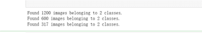
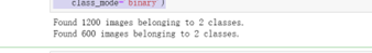
from tensorflow.keras.preprocessing.image import ImageDataGenerator

# 图片预处理参数
BATCH_SIZE = 20
IMG_SIZE = (150, 150)

# 归一化处理
datagen = ImageDataGenerator(rescale=1./255)

# 训练集生成器
train_dir = 'D:/python/train'
train_generator = datagen.flow_from_directory(
    train_dir,
    target_size=IMG_SIZE,
    batch_size=BATCH_SIZE,
    color_mode='rgb',
    class_mode='binary')

# 验证集生成器
validation_dir = 'D:/python/validation'
validation_generator = datagen.flow_from_directory(
    validation_dir,
    target_size=IMG_SIZE,
    batch_size=BATCH_SIZE,
    color_mode='rgb',
    class_mode='binary')

# 测试集生成器
test_dir = 'D:/python/test'
test_generator = datagen.flow_from_directory(
    test_dir,
    target_size=IMG_SIZE,
    batch_size=BATCH_SIZE,
    color_mode='rgb',
    class_mode='binary')
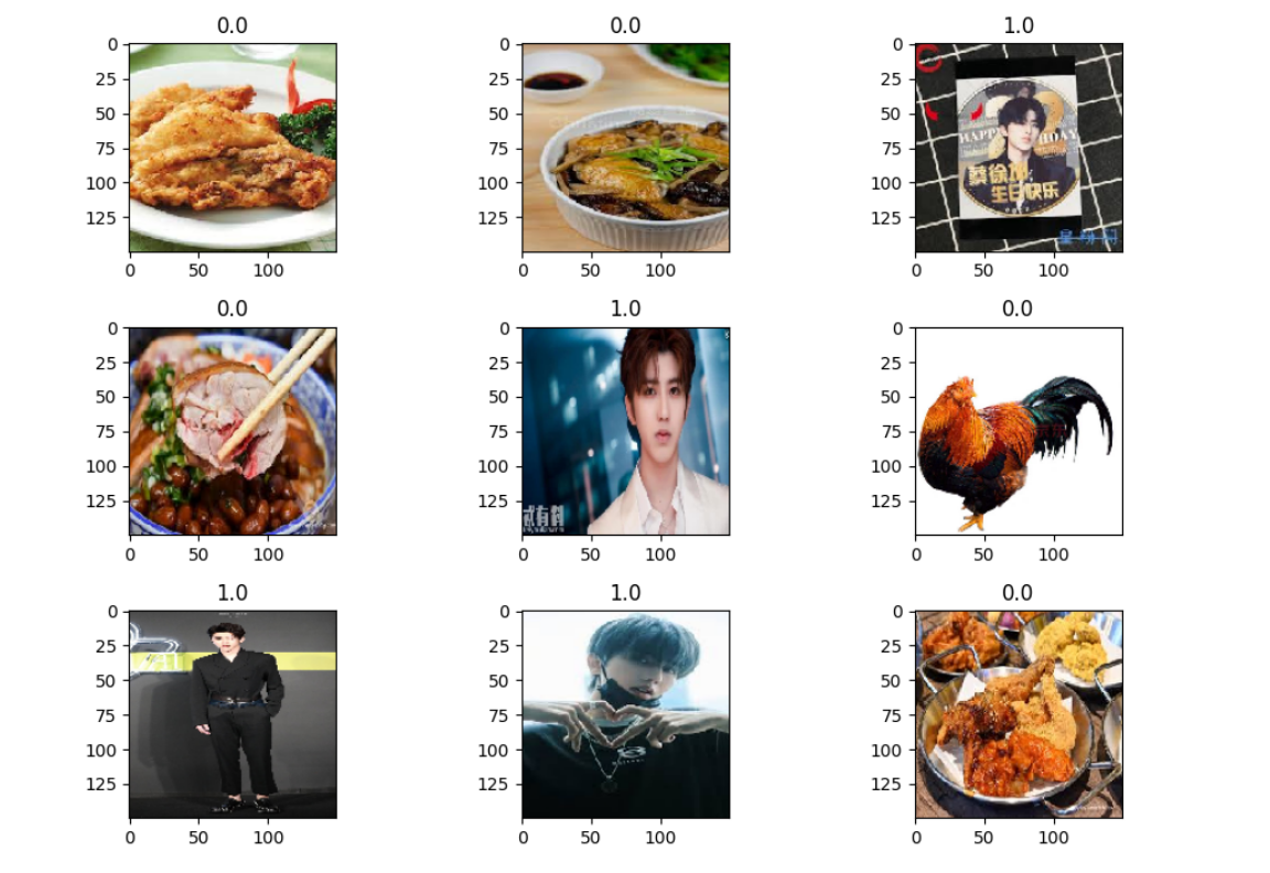
6.查看经过处理的图片以及它的binary标签
# 查看经过处理的图片以及它的binary标签
fit, ax = plt.subplots(nrows=3, ncols=3, figsize=(10, 7))

for i, a in enumerate(ax.flat):
    img, label = test_generator.next()
    a.imshow(img[0],)
    a.set_title(label[0])

plt.tight_layout()
plt.show()
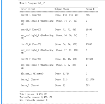
7.构建神经网络并对模型进行训练
from tensorflow.keras import optimizers

# 构建神经网络
model = models.Sequential()
# 1.Conv2D层,32个过滤器。输出图片尺寸:150-3+1=148*148,参数数量:32*3*3*3+32=896
model.add(layers.Conv2D(32, (3, 3),
                        activation='relu',
                        input_shape=(150, 150, 3)))  # 卷积层1
model.add(layers.MaxPooling2D((2, 2)))  # 最大值池化层1。输出图片尺寸:148/2=74*74

# 2.Conv2D层,64个过滤器。输出图片尺寸:74-3+1=72*72,参数数量:64*3*3*32+64=18496
model.add(layers.Conv2D(64, (3, 3),
                        activation='relu'))  # 卷积层2
model.add(layers.MaxPooling2D((2, 2)))  # 最大值池化层2。输出图片尺寸:72/2=36*36

# 3.Conv2D层,128个过滤器。输出图片尺寸:36-3+1=34*34,参数数量:128*3*3*64+128=73856
model.add(layers.Conv2D(128, (3, 3),
                        activation='relu'))  # 卷积层3
model.add(layers.MaxPooling2D((2, 2)))  # 最大值池化层3。输出图片尺寸:34/2=17*17

# 4.Conv2D层,128个过滤器。输出图片尺寸:17-3+1=15*15,参数数量:128*3*3*128+128=147584
model.add(layers.Conv2D(128, (3, 3),
                        activation='relu'))  # 卷积层4
model.add(layers.MaxPooling2D((2, 2)))  # 最大值池化层4。输出图片尺寸:15/2=7*7

# 将输入层的数据压缩成1维数据,全连接层只能处理一维数据
model.add(layers.Flatten())

# 全连接层
model.add(layers.Dense(512,
                       activation='relu'))  # 全连接层1
model.add(layers.Dense(1,
                       activation='sigmoid'))  # 全连接层2,作为输出层。sigmoid分类,输出是两类别

# 编译模型
# RMSprop 优化器。因为网络最后一层是单一sigmoid单元,
# 所以使用二元交叉熵作为损失函数
# 编译模型
model.compile(loss='binary_crossentropy',
              optimizer=optimizers.RMSprop(lr=1e-4),
              metrics=['acc'])


# 看一下特征图的维度如何随着每层变化
model.summary()
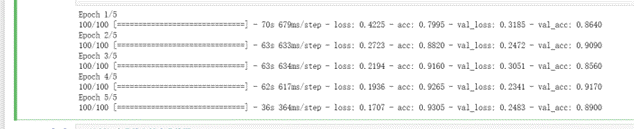
import itertools

# 训练模型5轮次
history_save = model.fit(
                    itertools.cycle(train_generator),
                    steps_per_epoch=100,
                    epochs=5,
                    validation_data=itertools.cycle(validation_generator),
                    validation_steps=50)
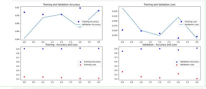
8.绘制损失曲线和精度曲线图
# 绘制损失曲线和精度曲线图
accuracy = history_save.history['acc']  # 训练集精度
loss = history_save.history['loss']  # 训练集损失
val_loss = history_save.history['val_loss']  # 验证集精度
val_accuracy = history_save.history['val_acc']  # 验证集损失
plt.figure(figsize=(17, 7))

# 训练集精度和验证集精度曲线图图
plt.subplot(2, 2, 1)
plt.plot(range(len(accuracy)), accuracy, 'bo', label='Training Accuracy')
plt.plot(range(len(val_accuracy)), val_accuracy, label='Validation Accuracy')
plt.title('Training and Validation Accuracy')
plt.legend(loc='center right')

# 训练集损失和验证集损失图
plt.subplot(2, 2, 2)
plt.plot(range(len(loss)), loss, 'bo', label='Training Loss')
plt.plot(range(len(val_loss)), val_loss, label='Validation Loss')
plt.title('Training and Validation Loss')
plt.legend(loc='center right')

# 训练集精度和损失散点图
plt.subplot(2, 2, 3)
plt.scatter(range(len(accuracy)), accuracy, label="Training Accuracy", color='b', s=25, marker="o")
plt.scatter(range(len(loss)), loss, label="Training Loss", color='r', s=25, marker="o")
plt.title('Training : Accuracy and Loss')
plt.legend(loc='center right')

# 验证集精度和损失散点图
plt.subplot(2, 2, 4)
plt.scatter(range(len(val_accuracy)), val_accuracy, label="Validation Accuracy", color='b', s=25, marker="o")
plt.scatter(range(len(val_loss)), val_loss, label="Validation Loss", color='r', s=25, marker="o")
plt.title('Validation : Accuracy and Loss')
plt.legend(loc='center right')

plt.show()
9.用ImageDataGenerator数据增强
train_datagen = ImageDataGenerator(rescale=1./255,
                                   rotation_range=40,  # 将图像随机旋转40度
                                   width_shift_range=0.2,  # 在水平方向上平移比例为0.2
                                   height_shift_range=0.2,  # 在垂直方向上平移比例为0.2
                                   shear_range=0.2,  # 随机错切变换的角度为0.2
                                   zoom_range=0.2,  # 图片随机缩放的范围为0.2
                                   horizontal_flip=True,  # 随机将一半图像水平翻转
                                   fill_mode='nearest')  # 填充创建像素
validation_datagen = ImageDataGenerator(rescale=1./255)

train_generator = train_datagen.flow_from_directory(
    train_dir,
    target_size=IMG_SIZE,  # 输入训练图像尺寸
    batch_size=BATCH_SIZE,
    class_mode='binary')

validation_generator = validation_datagen.flow_from_directory(
    validation_dir,
    target_size=IMG_SIZE,
    batch_size=BATCH_SIZE,
    class_mode='binary')
10.随机选取测试集的图片进行预测
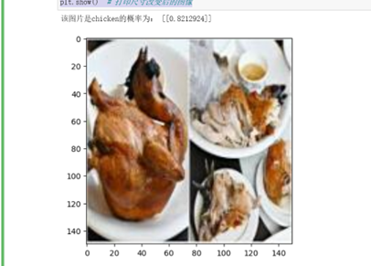
# 将图片缩小到(150,150)的大小
def convertjpg(jpgfile, outdir, width=150, height=150):
    img = Image.open(jpgfile)
    try:
        new_img = img.resize((width, height), Image.BILINEAR)
        new_img.save(os.path.join(outdir, os.path.basename(jpgfile)))
    except Exception as e:
        print(e)

# 从测试集随机获取一张chicken图片
chicken_test = r'D:/python/test/chicken/'
chicken_test_list = os.listdir(chicken_test)
key = random.randint(0, len(chicken_test_list))
img_key = chicken_test_list[key]
jpg_file = os.path.join(chicken_test, img_key)
convertjpg(jpg_file, "D:/python/test")  # 图像大小改变到(150,150)
img_scale = plt.imread('D:/python/test/' + img_key)
plt.imshow(img_scale)  # 显示改变图像大小后的图片确实变到了(150,150)大小

# 调用训练模型结果进行预测
model = load_model('D:/python/zhi_model.h5')
img_scale = img_scale.reshape(1, 150, 150, 3).astype('float32')
img_scale = img_scale/255  # 归一化到0-1之间
result = model.predict(img_scale)  # 取图片信息
if result > 0.5:
    print('该图片是kun的概率为:', result)
else:
    print('该图片是chicken的概率为:', 1-result)
plt.show()  # 打印尺寸改变后的图像
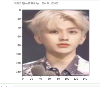
import cv2

# 自定义一张kun性图片进行预测
diy_img = 'D:/python/test/123.jpg'

img_scale = cv2.imread(diy_img)
img_scale = cv2.resize(img_scale, (150, 150))  # 调整图像大小为模型输入的大小
img_scale = cv2.cvtColor(img_scale, cv2.COLOR_BGR2RGB)  # 将图像从BGR通道顺序转换为RGB通道顺序

plt.imshow(img_scale)

# 调用数据增强后的训练模型结果进行预测
model = load_model('D:/python/zhi_model.h5')
img_scale = img_scale.reshape(1, 150, 150, 3).astype('float32')
img_scale = img_scale/255  # 归一化到0-1之间
result = model.predict(img_scale)  # 取图片信息
if result > 0.5:
    print('该图片是kun的概率为:', result)
else:
    print('该图片是chicken的概率为:', 1-result)
plt.show()
四、全部代码:
  1 import os
  2 import random
  3 from shutil import copy
  4 from matplotlib import pyplot as plt
  5 from keras import optimizers
  6 from keras import models
  7 from keras import layers
  8 from keras.preprocessing.image import ImageDataGenerator
  9 from keras.models import load_model
 10 from PIL import Image
 11
 12
 13 import os
 14 from shutil import copy
 15 # 定义路径和文件夹名
 16 base_dir = r'D:\python'
 17 train_dir = os.path.join(base_dir, 'train')
 18 validation_dir = os.path.join(base_dir, 'validation')
 19 test_dir = os.path.join(base_dir, 'test')
 20
 21 kun_train_dir = os.path.join(train_dir, 'kun')
 22 kun_validation_dir = os.path.join(validation_dir, 'kun')
 23 kun_test_dir = os.path.join(test_dir, 'kun')
 24
 25 chicken_train_dir = os.path.join(train_dir, 'chicken')
 26 chicken_validation_dir = os.path.join(validation_dir, 'chicken')
 27 chicken_test_dir = os.path.join(test_dir, 'chicken')
 28
 29 # 创建目录
 30 dir_list = [kun_train_dir, kun_validation_dir, kun_test_dir,
 31             chicken_train_dir, chicken_validation_dir, chicken_test_dir]
 32
 33 for dir_child in dir_list:
 34     os.makedirs(dir_child, exist_ok=True)
 35
 36 # 复制文件到不同目录
 37 def copy_files(source_path, destination_path, start_index, end_index):
 38     for i in range(start_index, end_index):
 39         child_path = os.path.join(source_path, os.listdir(source_path)[i])
 40         copy(child_path, destination_path)
 41
 42 # 复制kun图片
 43 kun_path = r'D:\zwc\ikun\坤坤\坤坤'
 44 kun_path_list = os.listdir(kun_path)
 45
 46 copy_files(kun_path, kun_train_dir, 0, 600)
 47 copy_files(kun_path, kun_validation_dir, 600, 900)
 48 copy_files(kun_path, kun_test_dir, 900, len(kun_path_list))
 49
 50 # 复制chicken图片
 51 chicken_path = r'D:\zwc\ikun\只因\只因'
 52 chicken_path_list = os.listdir(chicken_path)
 53
 54 copy_files(chicken_path, chicken_train_dir, 0, 600)
 55 copy_files(chicken_path, chicken_validation_dir, 600, 900)
 56 copy_files(chicken_path, chicken_test_dir, 900, len(chicken_path_list))
 57
 58 # 输出文件数量
 59 def print_file_count(path, label):
 60     print('total', label, 'images:', len(os.listdir(path)))
 61
 62 print_file_count(os.path.join(train_dir, 'kun'), 'training kun')
 63 print_file_count(os.path.join(train_dir, 'chicken'), 'training chicken')
 64
 65 print_file_count(os.path.join(validation_dir, 'kun'), 'validation kun')
 66 print_file_count(os.path.join(validation_dir, 'chicken'), 'validation chicken')
 67
 68 print_file_count(os.path.join(test_dir, 'kun'), 'test kun')
 69 print_file_count(os.path.join(test_dir, 'chicken'), 'test chicken')
 70
 71
 72
 73 # 查看图像以及对应的标签
 74 fit, ax = plt.subplots(nrows=3, ncols=3, figsize=(10, 7))
 75 # 查看图像的根路径
 76 test_view_path = r'D:\python\test\chicken'
 77 # 获取 test_view_path 下的文件夹列表
 78 test_view_list = os.listdir(test_view_path)
 79 for i, a in enumerate(ax.flat):
 80     view_path = os.path.join(test_view_path, test_view_list[i])
 81     # 读取源图
 82     a.imshow(plt.imread(view_path))
 83     # 添加图像名称
 84     a.set_title(chicken_path_list[i])
 85 plt.tight_layout()  # 自动调整子图参数,使之填充整个图像区域
 86 plt.show()
 87
 88
 89
 90 from tensorflow.keras.preprocessing.image import ImageDataGenerator
 91
 92 # 图片预处理参数
 93 BATCH_SIZE = 20
 94 IMG_SIZE = (150, 150)
 95
 96 # 归一化处理
 97 datagen = ImageDataGenerator(rescale=1./255)
 98
 99 # 训练集生成器
100 train_dir = 'D:/python/train'
101 train_generator = datagen.flow_from_directory(
102     train_dir,
103     target_size=IMG_SIZE,
104     batch_size=BATCH_SIZE,
105     color_mode='rgb',
106     class_mode='binary')
107
108 # 验证集生成器
109 validation_dir = 'D:/python/validation'
110 validation_generator = datagen.flow_from_directory(
111     validation_dir,
112     target_size=IMG_SIZE,
113     batch_size=BATCH_SIZE,
114     color_mode='rgb',
115     class_mode='binary')
116
117 # 测试集生成器
118 test_dir = 'D:/python/test'
119 test_generator = datagen.flow_from_directory(
120     test_dir,
121     target_size=IMG_SIZE,
122     batch_size=BATCH_SIZE,
123     color_mode='rgb',
124     class_mode='binary')
125
126
127
128 # 查看经过处理的图片以及它的binary标签
129 fit, ax = plt.subplots(nrows=3, ncols=3, figsize=(10, 7))
130
131 for i, a in enumerate(ax.flat):
132     img, label = test_generator.next()
133     a.imshow(img[0],)
134     a.set_title(label[0])
135
136 plt.tight_layout()
137 plt.show()
138
139
140
141 from tensorflow.keras import optimizers
142
143 # 构建神经网络
144 model = models.Sequential()
145 # 1.Conv2D层,32个过滤器。输出图片尺寸:150-3+1=148*148,参数数量:32*3*3*3+32=896
146 model.add(layers.Conv2D(32, (3, 3),
147                         activation='relu',
148                         input_shape=(150, 150, 3)))  # 卷积层1
149 model.add(layers.MaxPooling2D((2, 2)))  # 最大值池化层1。输出图片尺寸:148/2=74*74
150
151 # 2.Conv2D层,64个过滤器。输出图片尺寸:74-3+1=72*72,参数数量:64*3*3*32+64=18496
152 model.add(layers.Conv2D(64, (3, 3),
153                         activation='relu'))  # 卷积层2
154 model.add(layers.MaxPooling2D((2, 2)))  # 最大值池化层2。输出图片尺寸:72/2=36*36
155
156 # 3.Conv2D层,128个过滤器。输出图片尺寸:36-3+1=34*34,参数数量:128*3*3*64+128=73856
157 model.add(layers.Conv2D(128, (3, 3),
158                         activation='relu'))  # 卷积层3
159 model.add(layers.MaxPooling2D((2, 2)))  # 最大值池化层3。输出图片尺寸:34/2=17*17
160
161 # 4.Conv2D层,128个过滤器。输出图片尺寸:17-3+1=15*15,参数数量:128*3*3*128+128=147584
162 model.add(layers.Conv2D(128, (3, 3),
163                         activation='relu'))  # 卷积层4
164 model.add(layers.MaxPooling2D((2, 2)))  # 最大值池化层4。输出图片尺寸:15/2=7*7
165
166 # 将输入层的数据压缩成1维数据,全连接层只能处理一维数据
167 model.add(layers.Flatten())
168
169 # 全连接层
170 model.add(layers.Dense(512,
171                        activation='relu'))  # 全连接层1
172 model.add(layers.Dense(1,
173                        activation='sigmoid'))  # 全连接层2,作为输出层。sigmoid分类,输出是两类别
174
175 # 编译模型
176 # RMSprop 优化器。因为网络最后一层是单一sigmoid单元,
177 # 所以使用二元交叉熵作为损失函数
178 # 编译模型
179 model.compile(loss='binary_crossentropy',
180               optimizer=optimizers.RMSprop(lr=1e-4),
181               metrics=['acc'])
182
183
184 # 看一下特征图的维度如何随着每层变化
185 model.summary()
186
187
188
189 import itertools
190
191 # 训练模型5轮次
192 history_save = model.fit(
193                     itertools.cycle(train_generator),
194                     steps_per_epoch=100,
195                     epochs=5,
196                     validation_data=itertools.cycle(validation_generator),
197                     validation_steps=50)
198
199
200
201 # 绘制损失曲线和精度曲线图
202 accuracy = history_save.history['acc']  # 训练集精度
203 loss = history_save.history['loss']  # 训练集损失
204 val_loss = history_save.history['val_loss']  # 验证集精度
205 val_accuracy = history_save.history['val_acc']  # 验证集损失
206 plt.figure(figsize=(17, 7))
207
208 # 训练集精度和验证集精度曲线图图
209 plt.subplot(2, 2, 1)
210 plt.plot(range(len(accuracy)), accuracy, 'bo', label='Training Accuracy')
211 plt.plot(range(len(val_accuracy)), val_accuracy, label='Validation Accuracy')
212 plt.title('Training and Validation Accuracy')
213 plt.legend(loc='center right')
214
215 # 训练集损失和验证集损失图
216 plt.subplot(2, 2, 2)
217 plt.plot(range(len(loss)), loss, 'bo', label='Training Loss')
218 plt.plot(range(len(val_loss)), val_loss, label='Validation Loss')
219 plt.title('Training and Validation Loss')
220 plt.legend(loc='center right')
221
222 # 训练集精度和损失散点图
223 plt.subplot(2, 2, 3)
224 plt.scatter(range(len(accuracy)), accuracy, label="Training Accuracy", color='b', s=25, marker="o")
225 plt.scatter(range(len(loss)), loss, label="Training Loss", color='r', s=25, marker="o")
226 plt.title('Training : Accuracy and Loss')
227 plt.legend(loc='center right')
228
229 # 验证集精度和损失散点图
230 plt.subplot(2, 2, 4)
231 plt.scatter(range(len(val_accuracy)), val_accuracy, label="Validation Accuracy", color='b', s=25, marker="o")
232 plt.scatter(range(len(val_loss)), val_loss, label="Validation Loss", color='r', s=25, marker="o")
233 plt.title('Validation : Accuracy and Loss')
234 plt.legend(loc='center right')
235
236 plt.show()
237
238
239
240 train_datagen = ImageDataGenerator(rescale=1./255,
241                                    rotation_range=40,  # 将图像随机旋转40度
242                                    width_shift_range=0.2,  # 在水平方向上平移比例为0.2
243                                    height_shift_range=0.2,  # 在垂直方向上平移比例为0.2
244                                    shear_range=0.2,  # 随机错切变换的角度为0.2
245                                    zoom_range=0.2,  # 图片随机缩放的范围为0.2
246                                    horizontal_flip=True,  # 随机将一半图像水平翻转
247                                    fill_mode='nearest')  # 填充创建像素
248 validation_datagen = ImageDataGenerator(rescale=1./255)
249
250 train_generator = train_datagen.flow_from_directory(
251     train_dir,
252     target_size=IMG_SIZE,  # 输入训练图像尺寸
253     batch_size=BATCH_SIZE,
254     class_mode='binary')
255
256 validation_generator = validation_datagen.flow_from_directory(
257     validation_dir,
258     target_size=IMG_SIZE,
259     batch_size=BATCH_SIZE,
260     class_mode='binary')
261
262
263
264 # 将图片缩小到(150,150)的大小
265 def convertjpg(jpgfile, outdir, width=150, height=150):
266     img = Image.open(jpgfile)
267     try:
268         new_img = img.resize((width, height), Image.BILINEAR)
269         new_img.save(os.path.join(outdir, os.path.basename(jpgfile)))
270     except Exception as e:
271         print(e)
272
273 # 从测试集随机获取一张chicken图片
274 chicken_test = r'D:/python/test/chicken/'
275 chicken_test_list = os.listdir(chicken_test)
276 key = random.randint(0, len(chicken_test_list))
277 img_key = chicken_test_list[key]
278 jpg_file = os.path.join(chicken_test, img_key)
279 convertjpg(jpg_file, "D:/python/test")  # 图像大小改变到(150,150)
280 img_scale = plt.imread('D:/python/test/' + img_key)
281 plt.imshow(img_scale)  # 显示改变图像大小后的图片确实变到了(150,150)大小
282
283 # 调用训练模型结果进行预测
284 model = load_model('D:/python/zhi_model.h5')
285 img_scale = img_scale.reshape(1, 150, 150, 3).astype('float32')
286 img_scale = img_scale/255  # 归一化到0-1之间
287 result = model.predict(img_scale)  # 取图片信息
288 if result > 0.5:
289     print('该图片是kun的概率为:', result)
290 else:
291     print('该图片是chicken的概率为:', 1-result)
292 plt.show()  # 打印尺寸改变后的图像
293
294
295
296 import cv2
297
298 # 自定义一张kun性图片进行预测
299 diy_img = 'D:/python/test/123.jpg'
300
301 img_scale = cv2.imread(diy_img)
302 img_scale = cv2.resize(img_scale, (150, 150))  # 调整图像大小为模型输入的大小
303 img_scale = cv2.cvtColor(img_scale, cv2.COLOR_BGR2RGB)  # 将图像从BGR通道顺序转换为RGB通道顺序
304
305 plt.imshow(img_scale)
306
307 # 调用数据增强后的训练模型结果进行预测
308 model = load_model('D:/python/zhi_model.h5')
309 img_scale = img_scale.reshape(1, 150, 150, 3).astype('float32')
310 img_scale = img_scale/255  # 归一化到0-1之间
311 result = model.predict(img_scale)  # 取图片信息
312 if result > 0.5:
313     print('该图片是kun的概率为:', result)
314 else:
315     print('该图片是chicken的概率为:', 1-result)
316 plt.show()
五、实验总结
机器学习就是通过利用数据,训练模型,然后模型预测的一种方法。这次学习主要是对二分类进行实践。二分类:所用到的二分类函数即sigmoid。用ImageDataGenerator数据增强进行训练。绘制训练的损失精度曲线图。训练模型精度较低。但对图像进行识别的精确率仍是较准确的。
本次程序设计的不足:在数据增强上效果不是很明显,在设计过程中还遇到图像失真导致训练精度上升缓慢。
改进:可以进行多次训练,提高次数