
第三周:卷积神经网络 part 2
第三周:卷积神经网络 part 2
问题总结
-
输出层激活函数是否有必要?
-
为什么DnCNN要输出残差图片?图像复原又该如何操作?
-
DSCMR中的J2损失函数效果并不明显,为什么还要引入呢?
代码练习
MobileNet V1
Mobilenet v1是Google于2017年发布的网络架构,旨在充分利用移动设备和嵌入式应用的有限的资源,有效地最大化模型的准确性,以满足有限资源下的各种应用案例。
使用了深度可分离卷积,把标准卷积分解为 depth-wise 和 point-wise 卷积,合起来被称作Depthwise Separable Convolution(参见Google的Xception)。
将常规卷积的做法(改变大小和通道数)拆分成两步走:depthwise层,只改变feature map的大小,不改变通道数;Pointwise 层,只改变通道数,不改变大小。
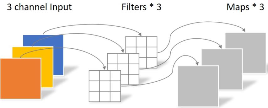
该结构和常规卷积操作类似,可用来提取特征,但相比于常规卷积操作,其参数量和运算成本较低。所以在一些轻量级网络中会碰到这种结构如MobileNet。
class Block(nn.Module):
    '''Depthwise conv + Pointwise conv'''
    def __init__(self, in_planes, out_planes, stride=1):
        super(Block, self).__init__()
        # Depthwise 卷积,3*3 的卷积核,分为 in_planes,即各层单独进行卷积
        self.conv1 = nn.Conv2d(in_planes, in_planes, kernel_size=3, stride=stride, padding=1, groups=in_planes, bias=False)
        self.bn1 = nn.BatchNorm2d(in_planes)
        # Pointwise 卷积,1*1 的卷积核
        self.conv2 = nn.Conv2d(in_planes, out_planes, kernel_size=1, stride=1, padding=0, bias=False)
        self.bn2 = nn.BatchNorm2d(out_planes)

    def forward(self, x):
        out = F.relu(self.bn1(self.conv1(x)))
        out = F.relu(self.bn2(self.conv2(out)))
        return out
MobileNet V1网络:
class MobileNetV1(nn.Module):
    # (128,2) means conv planes=128, stride=2
    cfg = [(64,1), (128,2), (128,1), (256,2), (256,1), (512,2), (512,1),
           (1024,2), (1024,1)]

    def __init__(self, num_classes=10):
        super(MobileNetV1, self).__init__()
        self.conv1 = nn.Conv2d(3, 32, kernel_size=3, stride=1, padding=1, bias=False)
        self.bn1 = nn.BatchNorm2d(32)
        self.layers = self._make_layers(in_planes=32)
        self.linear = nn.Linear(1024, num_classes)

    def _make_layers(self, in_planes):
        layers = []
        for x in self.cfg:
            out_planes = x[0]
            stride = x[1]
            layers.append(Block(in_planes, out_planes, stride))
            in_planes = out_planes
        return nn.Sequential(*layers)

    def forward(self, x):
        out = F.relu(self.bn1(self.conv1(x)))
        out = self.layers(out)
        out = F.avg_pool2d(out, 2)
        out = out.view(out.size(0), -1)
        out = self.linear(out)
        return out
经过10轮训练后,对CIFAR10数据集的表现如下:
Accuracy of the network on the 10000 test images: 78.14 %
可以看出MoblieNet在降低参数量的同时仍保持了较好的准确率。
MobileNet V2
Mark Sandler在CVPR 2018提出了MobileNetV2。
-
MobileNet V1 的主要问题:
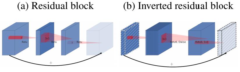
- 结构非常简单,但是没有使用RestNet里的residual learning
- Depthwise Conv确实是大大降低了计算量,但实际中,发现不少训练出来的kernel是空的
-
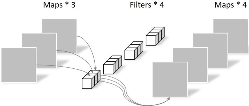
MobileNet V2 的主要改动:
- 设计了Inverted residual block
- 去掉输出部分的ReLU6
class Block(nn.Module):
    '''expand + depthwise + pointwise'''
    def __init__(self, in_planes, out_planes, expansion, stride):
        super(Block, self).__init__()
        self.stride = stride
        # 通过 expansion 增大 feature map 的数量
        planes = expansion * in_planes
        self.conv1 = nn.Conv2d(in_planes, planes, kernel_size=1, stride=1, padding=0, bias=False)
        self.bn1 = nn.BatchNorm2d(planes)
        self.conv2 = nn.Conv2d(planes, planes, kernel_size=3, stride=stride, padding=1, groups=planes, bias=False)
        self.bn2 = nn.BatchNorm2d(planes)
        self.conv3 = nn.Conv2d(planes, out_planes, kernel_size=1, stride=1, padding=0, bias=False)
        self.bn3 = nn.BatchNorm2d(out_planes)

        # 步长为 1 时,如果 in 和 out 的 feature map 通道不同,用一个卷积改变通道数
        if stride == 1 and in_planes != out_planes:
            self.shortcut = nn.Sequential(
                nn.Conv2d(in_planes, out_planes, kernel_size=1, stride=1, padding=0, bias=False),
                nn.BatchNorm2d(out_planes))
        # 步长为 1 时,如果 in 和 out 的 feature map 通道相同,直接返回输入
        if stride == 1 and in_planes == out_planes:
            self.shortcut = nn.Sequential()

    def forward(self, x):
        out = F.relu(self.bn1(self.conv1(x)))
        out = F.relu(self.bn2(self.conv2(out)))
        out = self.bn3(self.conv3(out))
        # 步长为1,加 shortcut 操作
        if self.stride == 1:
            return out + self.shortcut(x)
        # 步长为2,直接输出
        else:
            return out
MobileNet V2网络:
class MobileNetV2(nn.Module):
    # (expansion, out_planes, num_blocks, stride)
    cfg = [(1,  16, 1, 1),
           (6,  24, 2, 1),
           (6,  32, 3, 2),
           (6,  64, 4, 2),
           (6,  96, 3, 1),
           (6, 160, 3, 2),
           (6, 320, 1, 1)]

    def __init__(self, num_classes=10):
        super(MobileNetV2, self).__init__()
        self.conv1 = nn.Conv2d(3, 32, kernel_size=3, stride=1, padding=1, bias=False)
        self.bn1 = nn.BatchNorm2d(32)
        self.layers = self._make_layers(in_planes=32)
        self.conv2 = nn.Conv2d(320, 1280, kernel_size=1, stride=1, padding=0, bias=False)
        self.bn2 = nn.BatchNorm2d(1280)
        self.linear = nn.Linear(1280, num_classes)

    def _make_layers(self, in_planes):
        layers = []
        for expansion, out_planes, num_blocks, stride in self.cfg:
            strides = [stride] + [1]*(num_blocks-1)
            for stride in strides:
                layers.append(Block(in_planes, out_planes, expansion, stride))
                in_planes = out_planes
        return nn.Sequential(*layers)

    def forward(self, x):
        out = F.relu(self.bn1(self.conv1(x)))
        out = self.layers(out)
        out = F.relu(self.bn2(self.conv2(out)))
        out = F.avg_pool2d(out, 4)
        out = out.view(out.size(0), -1)
        out = self.linear(out)
        return out
经过10轮训练后,对CIFAR10数据集的表现如下:
Accuracy of the network on the 10000 test images: 80.10 %
可以看出MoblieNet V2相对V1准确率有所提升。
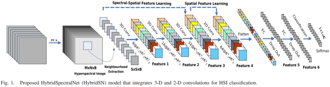
HybridSN 高光谱分类
构建一个混合网络解决高光谱图像分类问题,首先用3D卷积,然后使用2D卷积。
实验若设置对照(3D->2D,2D->3D),更具说服力。
一维卷积、二维卷积、三维卷积的区别:卷积神经网络(CNN)之一维卷积、二维卷积、三维卷积详解
class HybridSN(nn.Module):

  def __init__(self):
    super(HybridSN, self).__init__()
    # 3个3D卷积
    # conv1:(1, 30, 25, 25), 8个 7x3x3 的卷积核 ==> (8, 24, 23, 23)
    self.conv1_3d = nn.Conv3d(1,8,(7,3,3))
    self.relu1 = nn.ReLU()
	# conv2:(8, 24, 23, 23), 16个 5x3x3 的卷积核 ==>(16, 20, 21, 21)
    self.conv2_3d = nn.Conv3d(8,16,(5,3,3))
    self.relu2 = nn.ReLU()
	# conv3:(16, 20, 21, 21),32个 3x3x3 的卷积核 ==>(32, 18, 19, 19)
    self.conv3_3d = nn.Conv3d(16,32,(3,3,3))
    self.relu3 = nn.ReLU()
    # 2D卷积
	# conv4:(576, 19, 19),64个 3x3 的卷积核 ==>(64, 17, 17)
    self.conv4_2d = nn.Conv2d(576,64,(3,3))
    self.relu4 = nn.ReLU()
	# 接下来依次为256,128节点的全连接层,都使用比例为0.4的 Dropout
    self.fn1 = nn.Linear(18496,256)
    self.fn2 = nn.Linear(256,128)

    self.fn_out = nn.Linear(128,class_num)

    self.drop = nn.Dropout(p = 0.4)

    # self.soft = nn.Softmax(dim = 1)

  def forward(self, x):
    out = self.conv1_3d(x)
    out = self.relu1(out)
    out = self.conv2_3d(out)
    out = self.relu2(out)
    out = self.conv3_3d(out)
    out = self.relu3(out)
	# 进行二维卷积,因此把前面的 32*18 reshape 一下,得到 (576, 19, 19)
    b,x,y,m,n = out.size()
    out = out.view(b,x*y,m,n)

    out = self.conv4_2d(out)
    out = self.relu4(out)
	# 接下来是一个 flatten 操作,变为 18496 维的向量
    # 进行重组,以b行,d列的形式存放(d自动计算)
    out = out.reshape(b,-1)

    out = self.fn1(out)
    out = self.drop(out)
    out = self.fn2(out)
    out = self.drop(out)

    out = self.fn_out(out)

    # out = self.soft(out)

    return out
accuracy 0.9740 9225
还可以继续提升性能:增大训练样本、调节学习率。
论文阅读心得
Beyond a Gaussian Denoiser(DnCNN)
第一次在图像去噪领域使用深度学习方法。
原来多用bm3d。
该论文提出了卷积神经网络结合残差学习来进行图像降噪,直接学习图像噪声,可以更好的降噪。
- 强调了residual learning(残差学习)和batch normalization(批量标准化)在图像复原中相辅相成的作用,可以在较深的网络的条件下,依然能带来快的收敛和好的性能。
- 文章提出DnCNN,在高斯去噪问题下,用单模型应对不同程度的高斯噪音;甚至可以用单模型应对高斯去噪、超分辨率、JPEG去锁三个领域的问题。
摘自:【图像去噪】DnCNN论文详解(Beyond a Gaussian Denoiser: Residual Learning of Deep CNN for Image Denoising)
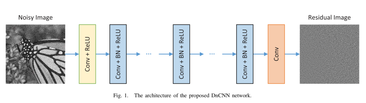
全卷积,将DnCNN的卷积核大小设置为3 * 3,并且去掉了所有的池化层。
内部协变量移位(internal covariate shift):深层神经网络在做非线性变换前的激活输入值,随着网络深度加深或者在训练过程中,其分布逐渐发生偏移或者变动,之所以训练收敛慢,一般是整体分布逐渐往非线性函数的取值区间的上下限两端靠近(对于Sigmoid函数来说,意味着激活输入值WU+B是大的负值或正值),所以这导致反向传播时低层神经网络的梯度消失,这是训练深层神经网络收敛越来越慢的本质原因。
批量标准化(batch normalization):就是通过一定的规范化手段,把每层神经网络任意神经元这个输入值的分布强行拉回到均值为0方差为1的标准正态分布,即把越来越偏的分布强制拉回比较标准的分布,这样使得激活输入值落在非线性函数对输入比较敏感的区域,所以输入的小变化才就会导致损失函数有较大的变化,意思就是让梯度变大,避免梯度消失问题产生,而且梯度变大意味着学习收敛速度快,能大大加快训练速度。
- BN的作用:
在每一层的非线性处理之前加入标准化、缩放、移位操作来减轻内部协变量的移位。可以给训练带来更快的速度,更好的表现,使网络对初始化变量的影响没有那么大。
- 实验部分:
- 对比有无residual learning与batch normalization对复原效果、收敛快慢的影响,最终证明这两是相辅相成的,都利用上时网络各方面性能达到最好。
- 根据特定程度的高斯噪声训练DnCNN-S、根据不定程度的高斯噪声训练DnCNN-B、根据不同程度的噪音(包括不同程度的高斯噪声、不同程度的低分辨率、不同程度的JPEG编码)训练的DnCNN-3来与最前沿的其他算法做对比实验。结论:DnCNN-S有最好的性能,但是DnCNN-B也有优于其他算法的性能,证明了DnCNN-B具有很好的盲去高斯噪声的能力;DnCNN-3则证明了DnCNN-3具有不俗的复原图像的泛化能力。
- 对比了DnCNN与其他前沿去噪算法的运行速度的实验,结论:速度还是不错的,CPU\GPU环境下均属于中上水平。
SENet
国内自动驾驶创业公司 Momenta 在 ImageNet 2017 挑战赛中夺冠,网络架构为 SENet,论文作者为 Momenta 高级研发工程师胡杰。该网络通过学习的方式获取每个特征通道的重要程度,然后依照这个重要程度去提升有用的特征并抑制对当前任务用处不大的特征。
引入注意力机制:强调重要部分(深色部分),忽略不重要部分(浅色部分)。
类似的还有双重注意力网络(DANet)等。
可以在不同维度上进行压缩,设置对照。
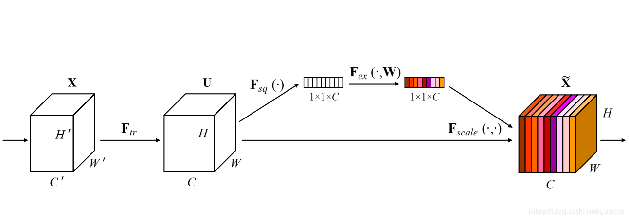
SENet的全称是Squeeze-and-Excitation Networks(压缩和激励网络),主要由两部分组成:
- Squeeze部分。即为压缩部分,原始feature map的维度为H×W×C,其中H是高度(Height),W是宽度(width),C是通道数(channel)。Squeeze做的事情是把H×W×C压缩为1×1×C,相当于把H×W压缩成一维了,实际中一般是用global average pooling实现的。H×W压缩成一维后,相当于这一维参数获得了之前H×W全局的视野,感受区域更广。
- Excitation部分。得到Squeeze的1×1×C的表示后,加入一个FC全连接层(Fully Connected),对每个通道的重要性进行预测,得到不同channel的重要性大小后再作用(激励)到之前的feature map的对应channel上,再进行后续操作。
可以看出,SENet和ResNet很相似,但比ResNet做得更多。ResNet只是增加了一个skip connection,而SENet在相邻两层之间加入了处理,使得channel之间的信息交互成为可能,进一步提高了网络的准确率。
SE模块主要为了提升模型对channel特征的敏感性,这个模块是轻量级的,而且可以应用在现有的网络结构中,只需要增加较少的计算量就可以带来性能的提升。
深度监督跨模态检索(DSCMR)
该论文设计了三个损失函数,用来提升深度跨模态检索的准确率。
J2损失函数使用数学公式推导,但效果并不明显。

 浙公网安备 33010602011771号