
Chapter 4: Supervised Learning
Acknowledgment: Most of the knowledge comes from Yuan Yang's course "Machine Learning".
Linear Regression
就是一个很传统的统计学任务。
用最小二乘法可知,\(w^* = (X^\top X)^{-1}X^{\top}Y\). But the inverse is hard to compute.
We can use gradient descent. Define the square loss:
What if the task is not regression but classification?
Consider binary classification at first. A naive way is to use positive and negative to represent 2 classes. However, the gradient can not give meaningful gradient information.
方法一:没有导数我就设计一种不需要导数信息的算法——感知机
方法二:把硬的变软,人为创造出导数——logistics regression
Perceptron
Intuition: adding \(x\) to \(w\) will make \(w^x\) larger.
Limitation: it can only learn linear functions, so it does not converge if data is not linearly separable.
Update rule: Adjust \(w\) only when make mistakes. If \(y > 0\) and \(wx<0\):
If \(y < 0\) and \(wx>0\):
combine these 2 into if \(ywx < 0\) \((y_i \in \{-1, +1\})\)
Convergence Proof:
Assume \(\|w^*\| = 1\) and \(\exist ~\gamma > 0 ~~ \text{s.t.} ~~ \forall ~ i ~~ y_i w^*x_i \ge \gamma\).
And \(\|x_i\| \le R\). Then at most \(\frac{R^2}{\gamma^2}\) mistakes.
Start from \(w_0 = 0\) Telescoping
Then
On the other hand:
Telescoping:
So
Logistic Regression(逻辑回归)
将分类问题转化为概率的回归问题。
Instead of using a sign function, we can output a probability. Here comes the important thought we have used in matrix completion. Relaxation!!!
Make the hard function \(\text{sign}(z)\) soft:
It remains to define a loss function. L1 and L2 are both not good enough, let's come to cross entropy:
Explanation:
-
We already know the actual probability distribution \(y\).
-
We estimate the difference of \(p_i\) and \(y_i\).
feature learning
Linear regression/classification can learn everything!
- If the feature is correct
In general, linear regression is good enough, but feature learning is hard
Deep learning is also called “representation learning” because it learns features automatically.
- The last step of deep learning is always linear regression/classification!
Regularization
This is a trick to avoid overfitting.
Ridge regression
This is \(\lambda\)-strongly convex.
An intuitive illustration of how this works. For each gradient descent step, split it into two parts:
- Part 1: Same as linear regression
- Part 2: “Shrink” every coordinate by \((1-\eta \lambda)\) (weight decay is a very important trick today)
Until two parts “cancel” out, and achieves equilibrium.
However, ridge regression can not find important features. It is essentially linear regression + weight decay.
Although the \(w\) vector will have a smaller norm, every feature may get some(possibly very small) weight
If we need to find important features, we need to optimize:
\(c\) means we want to ensure that there are at most \(c\) non-zero entries, i.e., those are themost important \(c\) features. Other features are not important.
Then relax "hard" to "soft" as we always do. Then we do LASSO regression:
LASSO regression
An intuitive illustration of how this works. For each gradient descent step, split it into two parts:
- Part 1: Same as linear regression
- Part 2: for every coordinate \(i\):\[\begin{equation} w_{t+1}^{(i)} = \begin{cases} \widehat{w}_{t}^{(i)}-\eta\lambda,&\text{for }\widehat{w}_{t}^{(i)} > \eta\lambda\\ \widehat{w}_{t}^{(i)}+\eta\lambda,&\text{for } \widehat{w}_{t}^{(i)}< -\eta\lambda\\ 0, &\text{for } \widehat{w}_{t}^{(i)} \in [-\eta\lambda, \eta\lambda] \end{cases} \end{equation} \]
Until two parts “cancel” out, and achieves equilibrium.
Compressed Sensing
Definition of RIP condition:
Let \(W \in \mathbb{R}^{n \times d}\) . \(W\) is \((\epsilon, s)\)-RIP if for all \(\|x\|_0 \leq s\), we have
This is called the Restricted Isometry Property (RIP). It means \(W\) is (almost) not expanding \(x\) towards any direction, as long as \(x\) is sparse. It is close to the identity matrix in the "sparse space of \(x\)," whatever it means.
Without the sparsity condition, this is impossible (think about \(W\)'s eigenspace; there exists an eigenvector with a \(0\) eigenvalue).
Naïve application for RIP (Theorem 1)
Theorem: Let \(\epsilon < 1\) and let \(W\) be a \((\epsilon, 2s)\)-RIP matrix. Let \(x\) be a vector such that \(\|x\|_0 \leq s\), let \(y = Wx\) be the compression of \(x\), and let
be a reconstructed vector. Then \(\tilde{x} = x\).
x is the only vector that gives y as the result after applying W under sparse conditions.
proof: 反证法 注意到是 \((\epsilon, 2s)\)-RIP
If not, i.e., \(\tilde{x} \neq x\). Since \(Wx = y\), we know \(\|\tilde{x}\|_0 \leq \|x\|_0 \leq s\), so \(\|x - \tilde{x}\|_0 \leq 2s\). We apply RIP condition on \(x - \tilde{x}\) and get
Notice that \(\|W(x - \tilde{x})\|_2^2 = 0\), and \(\|x - \tilde{x}\|_2^2 \neq 0\), so we have \(0 \leq (1-\epsilon) \leq 0 \leq (1+\epsilon)\), which is a contradiction.
这个定理还是有一样的问题,0阶不好优化,需要relax到一阶
Theorem2: 0-norm \(\rightarrow\) 1-norm
Let \(\epsilon < 1\) and let \(W\) be a \((\epsilon, 2s)\)-RIP matrix. Let \(x\) be a vector such that \(\|x\|_0 \leq s\), let \(y = Wx\) be the compression of \(x\), and \(\epsilon < \frac{1}{1 + \sqrt{2}}\). Then
Theorem 2 + x contains noise (Theorem 3)
Let \(\epsilon < \frac{1}{1+\sqrt{2}}\) and let \(W\) be a \((\epsilon, 2s)\)-RIP matrix.
Let \(x\) be an arbitrary vector and denote \(x_s \in \arg\min_{v: \|v\|_0 \leq s} \|x - v\|_1\).
That is, \(x_s\) is the vector which equals \(x\) on the \(s\) largest elements of \(x\) and equals \(0\) elsewhere.
Let \(y = Wx\) be the compression of \(x\) and let \(x^* \in \arg\min_{v: Wv = y} \|v\|_1\) be the reconstructed vector. Then:
where \(\rho = \frac{\sqrt{2}\epsilon}{1-\epsilon}\). When \(x = x_s\) (\(s\)-sparse), we get exact recovery \(x^* = x\).
Proof:
Before the proof, we need to clarify some notations.
Given a vector \(v\), a set of indices \(I\), denote \(v_I\) as the vector whose \(i\)th element is \(v_i\) if \(i \in I\), otherwise, the \(i\)th element is 0.
We partition indices as: \([d]=T_0 \cup T_1 \cup \ldots \cup T_{\frac{d}{s}-1}\). Each \(|T_i|=s\), and assume \(\frac{d}{s}\) is an integer for simplicity.
\(T_0\) contains the \(s\) largest elements in absolute value in \(x\). Then \(T_0^c=[d] \setminus T_0\).
\(T_1\) contains the \(s\) largest elements in \(h_{T_0^c}\). (not in \(x\)!). \(T_{0,1}=T_0 \cup T_1\) and \(T_{0,1}^c=[d] \setminus T_{0,1}\).
\(T_2\) contains the \(s\) largest elements in \(h_{T_{0,1}^c}\). \(T_3, T_4, \ldots\) are constructed in the same way.
Then based on our notation, \(\|x - x_s\|_1 = \|x_{T_0}^c\|_1\), 后面的证明只要都转到\(\|x_{T_0}^c\|_1\) 即可
Then begin our proof:
Let \(h=x^* - x\). We want to show that \(\|h\|_2\) is small.
We split \(h\) into two parts: \(h=h_{T_{0,1}} + h_{T_{0,1}^c}\).
\(h_{T_{0,1}}\) is \(2s\)-sparse, we move large elements inside, then use RIP to bound it.
\(h_{T_{0,1}^c}\) is the rest small entries, we use intuition (袁洋老师经典的棍子问题) to bound it.
Step1: bound \(\|h_{T_{0,1}^c}\|_2 \leq \|h_{T_0}\|_2 + 2s^{-1/2} \|x - x_s\|_1\)
The first inequality is by definition of infinity norm. Sum over \(j=2, 3, \ldots\) by triangle inequality, we have
We want to show \(\|h_{T_0^c}\|_1\) will not be too big.
解释一下这个式子(*): For any \(j > 1\), \(\forall i \in T_j\), \(i' \in T_{j-1}\), \(|h_i| \leq |h_{i'}|\) (by definition of \(T\)). So
Then we want to bound \(\|h_{T_0}^c\|_1\)。
\(x^* = x + h\) has minimal \(\ell_1\) norm in all vector satisfy \(Wx = y\), and \(x\) satisfies \(Wx = y\).
So:
因为我们等一下也要bound$ |h_{T_{0,1}}|_2 $ 所以这边放缩到这里,也是没有问题的。
总结一下,经过step1之后,我们得到了什么
Step2: Then we want to bound \(\|h_{T_{0,1}}\|_2\)
Use RIP condition bound these big terms:
The last equality is because \(Wh_{T_{0,1}} = Wh - \sum_{j \geq 2} W h_{T_j} = -\sum_{j \geq 2} W h_{T_j}\),
The final result is the inner products between disjoint index sets. We use a very useful lemma:
Theorem: Let \(W\) be \((\epsilon,2s)\)-RIP, \(\forall I, J\) disjoint sets of size \(\leq s\), for any vector \(\mu\) we have \(\langle Wu_I, Wu_J \rangle \leq \epsilon \|u_I\| \|u_J\|\)
proof of this small thm:
WLOG assume \(\|u_I\| = \|u_J\| = 1\).
We can bound these two terms by RIP condition:
Since \(|J \cup I| \leq 2s\), we get from RIP condition that (notice \(\langle u_I, u_J \rangle = 0\))
Now come back to the original proof.
Therefore, we have for \(i \in \{0, 1\}\), \(j \geq 2\): \(|\langle W h_{T_i}, W h_{T_j} \rangle| \leq \epsilon \|h_{T_i}\|_2 \|h_{T_j}\|_2\).
Continue:
\(\|h_{T_0}^c\|\) 我们是bound过的呀,但是这里又转到 \(\|h_{T_{0,1}}\|_2\),互相bound?这么奇怪。
Continue: 设$ \frac{\sqrt{2}\epsilon}{1-\epsilon} = \rho$
然后我们把这个再代入前面的式子:
这样就证完了。
How to construct a RIP matrix?
Random matrix
Theorem 4: Let \(U\) be an arbitrary fixed \(d \times d\) orthonormal matrix, let \(\epsilon, \delta\) be scalars in \((0,1)\). Let \(s\) be an integer in \([d]\), let \(n\) be an integer that satisfies:
Let \(W \in \mathbb{R}^{n \times d}\) be a matrix such that each element of \(W\) is distributed normally with zero mean and variance of \(1/n\). Then with a probability of at least \(1-\delta\) over the choice of \(W\), the matrix \(WU\) is \((\epsilon,s)\)-RIP.
解释:
-
Matrix \(U\) can be identity, so \(W\) is also \((\epsilon,s)\)-RIP.
-
Before we delve deeper into this proof, we discuss a question: Why is \(WU\) useful?
- \(y=Wx\), \(W\) is RIP, but \(x\) can not always be sparse.
- But also \(y=(WU)a\), \(WU\) is still RIP, \(U\) is orthonormal, \(a\) is sparse. 也就是可以加一个任意的正交的矩阵,将不sparse的输入变成sparse。
The rough idea of this proof is:
RIP condition holds for all possible (infinitely many) sparse vectors, but we want to apply union bound. So:
-
Continuous space \(\rightarrow{}\) finite number of points
-
Consider a specific index set \(I\) of size \(s\)(get this RIP condition on this specific index set)
-
Use this index set to enter the sparse space
-
Apply union bound over all possible \(I\)
Let's begin our proof:
Lemma 2:
Let \(\epsilon \in (0,1)\). There exists a finite set \(Q \subseteq \mathbb{R}^d\) of size \(|Q|\le (\frac{5}{\epsilon})^d\) such that:
意义:
我们能够用有限的点,覆盖一个高维空间(此处覆盖的意思是,高维空间中的任意一点,到我们取的有限的点集的最小距离,都很小)。也就是对应我们idea中的第一步——"Continuous space \(\rightarrow{}\) finite number of points"
Proof:
假设\(\epsilon = 1/k\). 把k上取整成整数,let
也就是\(Q'\)中的每个点,的所有坐标,都是\([-1, 1]\)之间的的2k+1分点上。那这样,空间中的任意一点都一定处在一个方格中,到方格顶点的距离,最大是\(\frac{1}{k} \le \epsilon\).
Clearly, \(|Q'| = (2k+1)^d\)(每个维度2k+1个点嘛).
We shall set \(Q = Q' \cap B_2(1)\), where \(B_2(1)\) is the unit \(L_2\) ball of \(\mathbb{R}^d\). 然后应该还有一些计算,会得到\((\frac{5}{\epsilon})^d\)这个答案。
JL lemma:
Let \(Q\) be a finite set of vectors in \(\mathbb{R}^d\). Let \(\delta \in (0,1)\) and \(n\) be an integer such that:
Then, with probability of at least \(1-\delta\) over a choice of a random matrix \(W \in \mathbb{R}^{n \times d}\) such that each element of \(W\) is independently distributed according to \(\mathcal{N}(0,1/n)\), we have:
意义:
-
这个定理已经就和我们最后要证的RIP的条件几乎一模一样了。只不过这里x不是sparse,而是在finite set中取。也就是对应我们idea中的第二步——"Consider a specific index set \(I\) of size \(s\)"
-
n的取值大小,和维数d没有关系了,只和finite set的size d有关,那么我们就可以用一个很小的Q和一个维数很低的n*d的矩阵W来做操作。
proof: omit here.
Lemma 3:
Let \(U\) be an orthonormal \(d \times d\) matrix and let \(I \subset [d]\) be a set of indices of size \(|I| = s\). Let \(S\) be the span of \(\{U_i : i \in I\}\), where \(U_i\) is the \(i\)-th column of \(U\). Let \(\delta \in (0,1)\), \(\epsilon \in (0,1)\), and \(n\) be an integer such that:
Then, with probability of at least \(1-\delta\) over a choice of a random matrix \(W \in \mathbb{R}^{n \times d}\) such that each element of \(W\) is independently distributed according to \(\mathcal{N}(0,1/n)\), we have:
意义:
lemma3已经非常接近我们最后要证的东西了,也就是对应idea中的第三步——"Use this index set to enter the sparse space"
首先解释一下: \(S\)是index的子集对应的多个列向量张成的向量空间,那其中的元素x,就是他们的线性组合,所以We can write \(x=U_Ia\) where \(a \in \mathbb{R}^s\)
If Lemma 3 is true, we know for any \(x \in S\),
Which implies that
因为a是unit length,所以我们只需要bound \(\|WU_Ia\|\)或者说\(\|Wx\|\)
只要lemma3正确,然后做第四步——"apply union bound over all possible \(I\)" (from \(\binom{d}{s}\)) i.e., \(\delta'=\delta \cdot d^s\),我们就证完了。
proof:
大致思路已经很清晰了,首先用JL lemma bound住离散的点\(v\)上的这个模长\(\|WU_Iv\|\),再用lemma2 bound从离散集合到全空间所有点的一个差距\(\|a-v\|\)也就是\(\|WU_I(a-v)\|\),那我们也就bound住了\(\|WU_Ia\|\).
It suffices to prove the lemma for all \(x \in S\) of the unit norm.
We can write \(x=U_Ia\) where \(a \in \mathbb{R}^s\), \(\|a\|_2=1\), and \(U_I\) is the matrix whose columns are \(\{U_i:i \in I\}\). 这里简单解释一下: 我前面说过,\(x\)是列向量的线性组合,所以写成了\(x=U_Ia\),又因为\(x\)和\(U\)的列向量都是unit length,\(U\)的列向量还相互之间正交,所以\(a\)也是unit length
Using Lemma 2 we know that there exists a set \(Q\) of size \(|Q| \leq (\frac{20}{\epsilon})^s\) such that:
Since \(U\) is orthonormal, we also have
也就是:
Apply JL lemma on \(\{U_Iv : v \in Q\}\), we know that for:
We can have:
This also implies
Let \(a\) be the smallest value such that for all \(x \in S\), \(\frac{\|Wx\|}{\|x\|} \leq 1+a\), clearly \(a < \infty\).(显然有上确界,然后设出来,然后求他) We want to show \(a < \epsilon\). This is the right half of the RIP condition.
\(\forall ~x \in S\) of unit norm, there exists \(v \in Q\) such that \(\|x - U_Iv\| \leq \epsilon/4\), and therefore
Notice that \(\|U_Iv\| \leq 1\), because \(U_I\) does not change length, and \(v\) is in \(Q\)(Q 肯定在单位球内). So
By definition of \(a\), we know
There may be some problem with the left half in PPT. TODO
Between this lemma 3 and the thm may be a gap, but 老师上课没讲。
作业中还有提到用random orthonormal basis 来构造RIP matrix的,这个在后面decision tree中会出现。
Support Vector Machine
概念解释
支持向量机(SVM)是一种二分类模型,它的基本模型是定义在特征空间上的间隔(margin)最大的线性分类器。
Margin: distance from the separator to the closest point
Samples on the margin are "support vectors".
数学表达式:
找到一个超平面\(wx+b=0\), s.t.
If the space is perfectly linear separable, this can be solved using quadratic programming in polytime.
那如果不是线性可分的呢?
Naïve answer:
\(\min \|w\|_2 + \lambda \cdot\) mistakes
i.e.
This is NP-Hard to minimize.
The indicator function is hard to optimize. Make it soft.
Relax the hard constraint:
\(\xi_i\) is a "slack variable".
"Violating the constraint" a little bit is OK. SVM with "Soft" margin.
This is called SVM with a "Soft" margin.
计算
Then we use "Dual" to solve SVM:
线性可分的情况:
Primal:
Dual:
Take derivative:
Plug it into \(L(w, \alpha)\), we get:
The relaxed case
Primal:
The Lagrangian:
where \(\alpha_i \geq 0\), \(\kappa_i \geq 0\)
Take derivative, we get the optimality conditions:
So, \(a_i = \lambda - \kappa_i \leq \lambda\). Here is one more constraint than the linearly separable case.
Then we put all the solution into \(L(w, b, \xi, a, \kappa)\):
The last formulation is the same as the linearly separable case.
kernel trick
We can use a kernel function to transform non-linearly separable into high dimensional space, in which the data is linearly separable.
Two problems:
-
kernal function \(\phi(x)\) dim too high, hard to compute.
-
The separator has a higher dim, hard to compute.
For \(\langle \phi(x_1), \phi(x_2)\rangle\), we can get it from \(\langle x_1, x_2 \rangle\). e.g. Quadratic kernel in PPT and Gauss kernel we always use.
\(\max \sum_i a_i - \frac{1}{2} \sum_i \sum_j y_i y_j a_i a_j \langle \phi(x_i), \phi(x_j) \rangle\)
- Only need to do \(n^2\) kernel computations \(\langle \phi(x_i), \phi(x_j) \rangle\)
When a new data point \(x\) comes, what do we do? Not computing \(\phi(x)\) -- can be expensive!
- \(w^T \phi(x) = \sum_i a_i y_i \langle \phi(x_i), \phi(x) \rangle\)
Assume \(r\) support vectors, then we only need to do at most \(r\) kernel computations
Therefore, no need for computing \(\phi(x)\)!
Move a step further, do we need to define \(\phi(x)\)?
Mercer’s Theorem: If the kernel matrix is positive semidefinite for any \(\{x_i\}\), then we know there exists \(\phi(\cdot)\) such that K is the kernel for \(\phi(\cdot)\)
That means we may define a \(K\) function for SVM, without knowing the exact format of \(\phi(\cdot)\)!!!
Decision Tree
pro: good explanations
con: big and deep, hard to switch, overfit easily.
前置知识
boolean function analysis: \(f:\{-1, 1\}^n \xrightarrow{} [0, 1]\)
Fourier basis of boolean function: \(\chi_S(x) = \prod_{i\in S}x_i, S\subset [n]\)
\(f(x) = \sum_{S} \hat{f}_S\chi_S(x), \hat{f}_S = \langle f, \chi_S(x)\rangle = E_{x\sim D}[f(x)\chi_S(x)]\)
\(L_1(f) = \sum_{S}|\hat{f}_S|\)
\(L_0 (f) = |{S:\hat{f}_S \ne 0}|\) sparsity 就是\(L_0(f)\)
A low degree means the degree of all its terms is bounded by this number. 也就是\(S\subset[n], |S| \le degree\)
Convert decision tree to low-degree sparse function
Thm: for any decision tree \(T\) with \(s\) leaf nodes, there exists a degree-\(\log {\frac{s}{\epsilon}}\) and sparsity-\(\frac{s^2}{\epsilon}\) function \(h\) that \(4\epsilon\)-approximates \(T\).
Proof:
Step 1: bounded its depth. Truncating \(T\) at depth \(\log \frac{s}{\epsilon}\)
This means there are at most \(\frac{s}{\epsilon}\) nodes remaining only when it is a full binary tree.
It differs by at most \(\frac{\epsilon}{s} \times s = \epsilon\). 这是为什么呢?因为走到每个最后一层的node的概率是\(\frac{\epsilon}{s}\),然后最多有s个node底下连到最终的leaves,也就是会被切掉。
(注意:这里已经造成了\(\epsilon\)的误差了)
So below we assume \(T\) has depth at most \(\log \frac{s}{\epsilon}\)
Step 2: bounded its degree and L1 norm
A tree with \(𝑠\) leaf nodes can be represented by union of \(𝑠\) “AND” terms
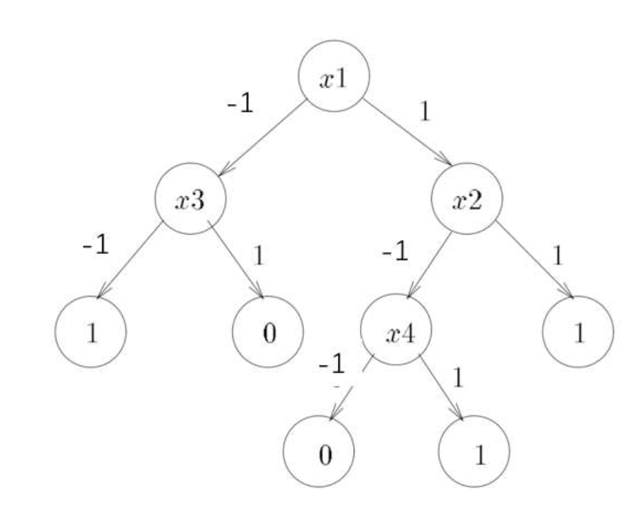
这是为什么呢?以下面这个图为例,假如我想要走到其中一个node,比如\(x_2\)右侧的那个1,必须\(x_1 =1, x_2 =1\), 那么这个node就可以被写成\(x_1 \wedge x_2\)
每个node都可以这样表示:\(\wedge_{i \in S} (x_i = \text{flag}_i), \text{flag}_i \in \{-1, 1\}\)
那么这个函数的各个系数分别是多少,可以用这个公式 \(\hat{f}_S = \langle f, \chi_S(x)\rangle = E_{x\sim D}[f(x)\chi_S(x)]\)进行计算。算出来一定刚好是
\(x_1 \wedge x_2 = \frac{1}{4}+\frac{1}{4}x_1 + \frac{1}{4}x_2 + \frac{1}{4}x_1 \cdot x_2\)
Because every AND term has \(L_1 = 1\) and at most \(\log \frac{s}{\epsilon}\) variables(depth is at most \(\log \frac{s}{\epsilon}\)), so \(L_1(f) \le s\) and degree of \(f\) bounded by \(\log \frac{s}{\epsilon}\)
Step 3
We need to prove:
For \(f\) s.t. \(L_1(f) \le s\) and degree at most \(\log \frac{s}{\epsilon}\), there is a function \(h\) with \(L_0 \le \frac{s^2}{\epsilon}\) s.t. \(E[(f-h)^2] \le \epsilon\).
Proof:
Let \(h\) include all terms in \(f\) s.t. \(|\hat{f}_S| \ge \frac{\epsilon}{L_1(f)}\). degree的条件肯定满足了.
这样的term最多只有\(L_1(f) / \frac{\epsilon}{L_1(f)} = \frac{L_1(f)^2}{\epsilon} \le \frac{s^2}{\epsilon}\). Sparsity的条件也满足了.
By Parseval identity, the missing term has a contribution at most:
这样误差的要求也满足。
上下两个误差相结合即可。
好了,现在我们已经把学一个决策树的问题转化为学一个函数的问题,而且这个函数在bool function basis上是low degree and sparse. 我们要怎么求这个函数在这组基分解上的系数呢?
Theoretically analysis
KM algorithm: (Not required)
Key point: recursively prune the less promising set of basis and explore a promising set of basis.
\(f_\alpha\) means the function of all the Fourier basis starting with \(\alpha\) summed together.
以一个由\(x_1, x_2, x_3\)三个变量的函数为例
All these functions are well defined and also satisfy parseval identity.
e.g.
Algorithm process:
def Coef(a):
If \(E[f^2_{a}] \ge \theta^2\):
If \(|a| = n\), then output \(a\) the degree can not be larger than n
Else Coef(a0); Coef(a1) // 感觉这也太暴力了吧qwq
大概就是只留下,系数比therohold大的节点,但是尽可能延展,然后又不会太长的节点。
当然这里大家肯定有疑问,我们要怎么样计算\(E[f^2_{a}]\)呢?
Lem3.2:
For any function \(f\), any \(1 \leq k < n\), any \(\alpha \in [-1, 1]^k\), and any \(x \in [-1, 1]^{n-k}\), \(f_\alpha (x) = \mathbb{E}_{y \in [-1,1]^k} \big[f(yx) \chi_\alpha (y)\big]\).
大概就是说,除了\(\alpha\)确定的那些bool变量,剩下的没有确定的bool变量,uniformly取所有可能,然后求均值。
This formulation implies that even though we do not know how to compute the value of \(𝑓_\alpha(𝑥)\) we can approximate it, by approximating the above expectation.
这个算法有two problem:
- Pretty slow
- Sequential algorithm, cannot be done in parallel
LMN Algorithm:
For every \(S\subset [n]\) with low degree, we estimate \(\hat{f}_S\) using \(m\) samples:
Do it for all \(S\) to get the function.
sample complexity is small and parallelizable.
Two problems:
- does not work well in practice
- does not have guarantees in the noisy setting.
From the point of view compressed sensing, we can control the error, because Fourier basis \(\{\chi_𝑆\}\) is a random orthonormal family.
Harmonica: compressed sensing
\(y = Ax\)
\(x\) is coefficient for \(X_s\), sparse in our case.
\(y\) 是整个函数的在不同取值下的结果,\(y_i = f(x_i)\)
\(A\): \(a_{ij}\) is \(X_{Sj}(x_i)\) 第i行代表的是第i个输入,第j列代表是第j个函数基的结果。
这个boolean function analysis是一个orthogonoal random matrix. 可以做compressed sensing 来复原\(x\) .
In practice, how to build a decision tree? Gini index
For a specific node, we have to distinguish a set of variables. Then we need to determine the next node.
We use the Gini index to measure the uncertainty of a variable relative to the decision outcome.
We pick the variable with the smallest Gini index/uncertainty.
Theoretically, if the decision tree is super deep, it can fit anything. But overfitting. We should avoid it, how? random forest.
Random forest (one of the best tools in practice)
Bagging
- Bagging是并行式集成学习方法最著名的代表。它直接基于自助采样法(bootstrap sampling)
随机森林是Bagging的一个扩展变体。
课件上面是说,我有放回的从原本的训练集中sample n次,构造一个大小一样的,但是(可能)有重复元素的集合。就相当于一个带权的子集。然后在这上面跑构造decision tree的算法。
重复B次,得到B个tree,然后取平均。
这样子的话,得到的tree会更稳定一些。
这还只是data bagging. 我们还可以做feature bagging,就是排除某些特征,来构造tree。这样也会更好。
• Each tree can only use a random subset of features
• So the decision tree is forced to use all possible information to predict,
instead of relying on a few powerful features
Boosting
We may have lots of weak learners. We want to combine them together to get a strong learner?
That is we want to learn a fixed combination of \(h_i\).
Adaboost
key idea: we can set the weight of each sample to control.
Constructing:
init: \(D_1(i) = \frac{1}{m}, \forall i\)
Given \(D_T\) and \(h_T\):
\(D_{t+1}(i) = \frac{D_t(i)}{Z_t} e^{-\alpha_t}\), if \(y_i = h_t(x_i)\) 答对了就减少权重
\(D_{t+1}(i) = \frac{D_t(i)}{Z_t} e^{\alpha_t}\), if \(y_i \ne h_t(x_i)\) 答错了就增大权重
\(Z_t = \sum_i D_t(i) e^{-\alpha_i y_i h_t(x_i)}\). Normalization factor.
\(\alpha_t = \frac{1}{2} \ln (\frac{1-\epsilon_t}{\epsilon_t})\ge 0\).
\(\epsilon_t\) 是错误率。
\(\alpha_t\)后面会讲为什么这么设定,也就是\(h_t\)的参数。错误率越小,权重越高,也很合理。
\(H_t = \text{sign} (\sum_t \alpha_t h_t (x))\)
Convergence Thm
Adaboost is adaptive: does not need to know \(\gamma\) or \(T\) as prior knowledge.
Convergence Proof
Step 1: unwrapping recurrence
Let \(f(x_i) = \sum_t\alpha_th_t(x_i)\), it becomes:
Step 2: bound error of H
Step 3: bound \(Z_T\)
对\(\alpha\) 求导,找到最小值\(\alpha_t = \frac{1}{2} \ln (\frac{1-\epsilon_t}{\epsilon_t})\), 所以\(Z_t = 2\sqrt{\epsilon_t(1-\epsilon_t)}\)
因为\(\epsilon_t = \frac{1}{2} - \gamma_t\)
From this Thm, we can know when \(T \xrightarrow{} +\infty, Error(H) \xrightarrow{} 0\). 但是这只是训练集的loss减小了,但是结合过多的weak learners容易过拟合。这就要讲接下来的这个部分 Margin-based analysis。
Margin-based analysis
Thm1: Let \(S\) be a sample of \(m\) samples chosen independently at random according to \(D\). Assume that the base hypothesis space \(H\) is finite, and let \(\delta > 0\). Then with probability at least \(1 - \delta\) over the random choice of the training set \(S\), every weighted average function \(f \in C\) satisfies the following bound for all \(\theta > 0\):
Define \(C_N\) to be the set of unweighted averages over \(N\) elements from \(H\)
We allow the same \(h \in H\) to appear multiple times in the sum. This set will play the role of the approximating set in the proof.
Any majority vote hypothesis \(f \in C\) can be associated with a distribution over \(H\) as defined by the coefficient \(a_h\). By choosing \(N\) elements of \(H\) independently at random according to this distribution we can generate an element of \(C_N\). Using such a construction we map each \(f \in C\) to a distribution \(Q\) over \(C_N\).
这边的思想还是很妙的。就是对于我的每一个函数f,我都构造一个函数集合的概率分布,这个函数集合的多个函数求均值等于f的值。
那么如何构造这个概率分布呢?\(f = \sum_i c_i h_i\), 那么\(h_i\)被采样到的概率,就是\(c_i\)。 这样去采样可以得到一个概率分布,而且\(C_N\)中的函数还是有限的,这是我们最关键。
Our goal is to upper bound the generalization error of \(f \in C\). For a fixed \(g \in C_N\) and \(𝜃 > 0\) we can separate this probability into two terms:
As this inequality holds for any \(g \in C_N\):
We first look at the second term:
Since \(f(x) = E_{g\sim Q}[g(x)]\), for a fixed sample \(x \sim D\), chernoff hoeffding bound can get:
Then we come to the first term:
Change a little bit of the statement, with a probability \(1 - \delta_N\), we have:
现在我们其实想bound的是,在已知\(P_{x\sim D, g\sim Q}[yg(x) \le \frac{\theta}{2}]\)的情况下,求\(P_{x\sim S, g\sim Q}[yg(x) > \frac{\theta}{2}]\)的概率下界。这就有点像已知realizable assumption,求取样复杂度。
To upper bound the first term, we use the union bound.
For any signle term, \(g\) and \(\theta\), 假设:
那么这个不等式成立的概率该怎么算呢?chernoff hoeffding bound
上面这个式子中的\(E\)是指\(E = E\Big[ P_{x\sim D, g\sim Q}[yg(x) > \frac{\theta}{2}]\Big]\)
然后遍历所有的\(|C_N| \le |H|^N\)还有所有的\(\theta\) 选择(\(\theta\) 只能是\(2i/N\) for \(i = 0, 1, ..., N\), 因为\(C_N\) 的构造方式)这个概率就变成了\((N+1)|C_N|e^{-2m\epsilon_N^2}\)
接着再对这个\(P[\cdot]\) 的概率不等式事件做等效变换:
最后这个式子的概率,应该小于\(\delta_N\)。 所以:
要保证最后这个不等是的话,由于\(|C_N| \le |H|^N\), 我们只需要保证
类似前面这个式子\(P_D[yf(x) \le 0] \le P_{x\sim D, g\sim Q}[yg(x) \le \frac{\theta}{2}] + P_{x\sim D, g\sim Q}[yg(x) > \frac{\theta}{2}|yf(x) \le 0]\)
我们有在\(S\) 上的一个式子
By chernoff hoeffding bound:
Combine them together, we can get for every \(\theta > 0\) and \(N \ge 1\):
将\(\epsilon_N\)代入,但是因为我们求的是任意的N,所以失败概率是被所有N取值的失败概率bound住的,\(\sum_{N}\delta_N = \delta, \delta_N = \frac{\delta}{N(N+1)}\)
最后再设置一下N的值,和\(\theta\) 有关。证毕,好长的定理啊。
Modification on Adaboost
Thm2:
Suppose the base learning algorithm, when called by AdaBoost, generates hypotheses with weighted training errors \(\epsilon_1, ⋯ , \epsilon_𝑇\). Then for any \(𝜃\), we have that:
Proof:
Note that if \(yf(x)\le \theta\), then (\(f(x) = \frac{\sum_t\alpha_th_t(x_i)}{\sum_t\alpha_t}\) here)
So:
因为\(\alpha_t = \frac{1}{2} \ln (\frac{1-\epsilon_t}{\epsilon_t})\), 所以:
这也是随着T指数级减小的。
Gradient Boosting
One drawback of adaboost: only cares about binary classification tasks.
What about regression tasks? We want to extend adaboost to regression tasks. Then we get gradient boosting.
Recall Adaboost is optimizing the following function:
- \(\prod_{t} Z_t = \frac{1}{m}\sum_i \exp\Big(-y_if(x_i)\Big) = \frac{1}{m}\sum_i \exp\Big(-y_i\sum_t \alpha_t h_t(x_i)\Big)\)
- This will go to 0 as T goes up
- How does it optimize? It uses coordinate descent
我们的需求是,给定了一些weak learners,我们要学一个他们的权重。
求一个全导数做gradient descent太贵了,因为weak learner数量可能是非常多的。
那就每次先固定所有其他的\(\alpha\) ,只学一个。
process:
- initially all \(\alpha_i = 0\)
- In each iteration of adaboost, we pick a coordinate \(\alpha_i\) and set it to make loss decrease most.
- It is like each time, we add a weak learning \(h\) into \(f\)
因为我们每次是往\(f\)中加一个weak learner,所以,所以我们加入的新函数可以在\((x_i, y_i - f(x_i))\) 做优化。
How is it related to gradient descent?
假如我们定义要优化的loss是 \(\mathcal{l}2\) loss:
如果做gradient descent,\(f_{t+1}(x_i) = f_t(x_i) -\eta\frac{\partial L}{\partial f(x_i)} = f_t(x_i) - \eta\big(f(x_i)-y_i\big) \rightarrow{} y_i\)那么更新之后就是更接近\(y\)
但是实际上,我每次不是更新\(\frac{\partial L}{\partial f(x_i)}\) 而是加一个\(\alpha_i h_i\). 效果也就只能勉强接近gradient descent
More generally, other losses are the same.


 浙公网安备 33010602011771号