为什么样本方差(sample variance)的分母是 n-1?
为什么样本方差(sample variance)的分母是 n-1?
(補充一句哦,題主問的方差 estimator 通常用 moments 方法估計。如果用的是 ML 方法,請不要多想不是你們想的那樣, 方差的 estimator 的期望一樣是有 bias 的,有興趣的同學可以自己用正態分佈算算看。)
本來,按照定義,方差的 estimator 應該是這個:
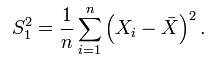
但,這個 estimator 有 bias,因為: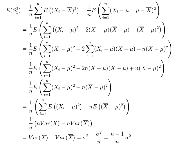
而 (n-1)/n * σ² != σ² ,所以,為了避免使用有 bias 的 estimator,我們通常使用它的修正值 S²: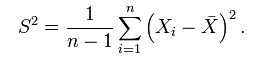
上面有答案解释得很明确,即样本方差计算公式里分母为的目的是为了让方差的估计是无偏的。无偏的估计(unbiased estimator)比有偏估计(biased estimator)更好是符合直觉的,尽管有的统计学家认为让mean square error即MSE最小才更有意义,这个问题我们不在这里探讨;不符合直觉的是,为什么分母必须得是
而不是
才能使得该估计无偏。我相信这是题主真正困惑的地方。
要回答这个问题,偷懒的办法是让困惑的题主去看下面这个等式的数学证明:.
但是这个答案显然不够直观(教材里面统计学家像变魔法似的不知怎么就得到了上面这个等式)。
下面我将提供一个略微更友善一点的解释。
==================================================================
===================== 答案的分割线 ===================================
==================================================================
首先,我们假定随机变量的数学期望
是已知的,然而方差
未知。在这个条件下,根据方差的定义我们有
由此可得.
因此是方差
的一个无偏估计,注意式中的分母不偏不倚正好是
!
这个结果符合直觉,并且在数学上也是显而易见的。
现在,我们考虑随机变量的数学期望
是未知的情形。这时,我们会倾向于无脑直接用样本均值
替换掉上面式子中的
。这样做有什么后果呢?后果就是,
如果直接使用作为估计,那么你会倾向于低估方差!
这是因为:
换言之,除非正好,否则我们一定有
,
而不等式右边的那位才是的对方差的“正确”估计!
这个不等式说明了,为什么直接使用会导致对方差的低估。
那么,在不知道随机变量真实数学期望的前提下,如何“正确”的估计方差呢?答案是把上式中的分母换成
,通过这种方法把原来的偏小的估计“放大”一点点,我们就能获得对方差的正确估计了:
至于为什么分母是而不是
或者别的什么数,最好还是去看真正的数学证明,因为数学证明的根本目的就是告诉人们“为什么”;暂时我没有办法给出更“初等”的解释了。
样本方差与样本均值,都是随机变量,都有自己的分布,也都可能有自己的期望与方差。取分母n-1,可使样本方差的期望等于总体方差,即这种定义的样本方差是总体方差的无偏估计。 简单理解,因为算方差用到了均值,所以自由度就少了1,自然就是除以(n-1)了。
再不能理解的话,形象一点,对于样本方差来说,假如从总体中只取一个样本,即n=1,那么样本方差公式的分子分母都为0,方差完全不确定。这个好理解,因为样本方差是用来估计总体中个体之间的变化大小,只拿到一个个体,当然完全看不出变化大小。反之,如果公式的分母不是n-1而是n,计算出的方差就是0——这是不合理的,因为不能只看到一个个体就断定总体的个体之间变化大小为0。
我不知道是不是说清楚了,详细的推导相关书上有,可以查阅。
因为样本均值与实际均值有差别。
如果分母用n,样本估计出的就方差会小于真实方差。
维基上有具体计算过程:
http://en.wikipedia.org/wiki/Unbiased_estimator#Sample_variance
Sample variance[edit]
The sample variance of a random variable demonstrates two aspects of estimator bias: firstly, the naive estimator is biased, which can be corrected by a scale factor; second, the unbiased estimator is not optimal in terms of mean squared error (MSE), which can be minimized by using a different scale factor, resulting in a biased estimator with lower MSE than the unbiased estimator. Concretely, the naive estimator sums the squared deviations and divides by n, which is biased. Dividing instead by n − 1 yields an unbiased estimator. Conversely, MSE can be minimized by dividing by a different number (depending on distribution), but this results in a biased estimator. This number is always larger than n − 1, so this is known as a shrinkage estimator, as it "shrinks" the unbiased estimator towards zero; for the normal distribution the optimal value is n + 1.
Suppose X1, ..., Xn are independent and identically distributed (i.i.d.) random variables with expectation μ and variance σ2. If the sample mean and uncorrected sample variance are defined as

then S2 is a biased estimator of σ2, because
![\begin{align}
\operatorname{E}[S^2]
&= \operatorname{E}\left[ \frac{1}{n}\sum_{i=1}^n \left(X_i-\overline{X}\right)^2 \right]
= \operatorname{E}\bigg[ \frac{1}{n}\sum_{i=1}^n \big((X_i-\mu)-(\overline{X}-\mu)\big)^2 \bigg] \\[8pt]
&= \operatorname{E}\bigg[ \frac{1}{n}\sum_{i=1}^n (X_i-\mu)^2 -
2(\overline{X}-\mu)\frac{1}{n}\sum_{i=1}^n (X_i-\mu) +
(\overline{X}-\mu)^2 \bigg] \\[8pt]
&= \operatorname{E}\bigg[ \frac{1}{n}\sum_{i=1}^n (X_i-\mu)^2 - (\overline{X}-\mu)^2 \bigg]
= \sigma^2 - \operatorname{E}\left[ (\overline{X}-\mu)^2 \right] < \sigma^2.
\end{align}](https://upload.wikimedia.org/math/5/5/7/5570b43693f45e8bba75ba5702a8fea5.png)
In other words, the expected value of the uncorrected sample variance does not equal the population variance σ2, unless multiplied by a normalization factor. The sample mean, on the other hand, is an unbiased[1] estimator of the population mean μ.
The reason that S2 is biased stems from the fact that the sample mean is an ordinary least squares (OLS) estimator for μ:  is the number that makes the sum
  as small as possible. That is, when any other number is plugged into this sum, the sum can only increase. In particular, the choice
  gives,

and then
![\begin{align}
\operatorname{E}[S^2]
&= \operatorname{E}\bigg[ \frac{1}{n}\sum_{i=1}^n (X_i-\overline{X})^2 \bigg]
< \operatorname{E}\bigg[ \frac{1}{n}\sum_{i=1}^n (X_i-\mu)^2 \bigg] = \sigma^2.
\end{align}](https://upload.wikimedia.org/math/7/7/c/77c63f4067f14b48b9fd59174a3f7948.png)
Note that the usual definition of sample variance is

and this is an unbiased estimator of the population variance. This can be seen by noting the following formula, which follows from the Bienaymé formula, for the term in the inequality for the expectation of the uncorrected sample variance above:
![\operatorname{E}\big[ (\overline{X}-\mu)^2 \big] = \frac{1}{n}\sigma^2 .](https://upload.wikimedia.org/math/2/e/7/2e70cecd544b2ee2e34415a0caa52d2f.png)
The ratio between the biased (uncorrected) and unbiased estimates of the variance is known as Bessel's correction.

 浙公网安备 33010602011771号