文献学习Speeding Up Assumption-Based SAT

Speeding Up Assumption-Based SAT

Hickey R., Bacchus F. (2019) Speeding Up Assumption-Based SAT. In: Janota M., Lynce I. (eds) Theory and Applications of Satisfiability Testing – SAT 2019. SAT 2019. Lecture Notes in Computer Science, vol 11628. Springer, Cham. https://doi.org/10.1007/978-3-030-24258-9_11

对应2020SAT竞赛求解器：

Abstract—This document describes Cadical-trail, Cadicalalluip,
Cadical-alluip-trail and Maple-LCM-Dist-alluip-trail
where two novel techniques ”trail-saving” and ”stable-allUIP”
are implemented.

 

---

 

Abstract

Assumption based SAT solving is an essential tool in many applications of SAT solving, especially in incremental SAT solving. For example, assumption based SAT solving is used when solving MaxSat, when computing minimal unsatisfiable subsets and minimal correction sets, and in various inductive verification applications. 译文：基于假设的SAT求解是许多SAT求解应用中必不可少的工具，尤其是增量式SAT求解。例如，在求解MaxSat时，在计算最小不可满足子集和最小修正集时，以及在各种归纳验证应用中使用基于假设的SAT求解。 The MiniSat SAT solver introduced a simple technique for extending a SAT solver to allow it to handle assumptions by forcing the SAT solver to make the assumed literals its initial decisions. 译文：MiniSat SAT求解器引入了一种简单的技术，用于扩展SAT求解器，使其能够通过强制SAT求解器做出其初始决策的假定文字来处理假设。   This approach persists in almost all current SAT solvers making it the most commonly used technique for handling assumptions.译文：这种方法一直存在于几乎所有的当前SAT求解器中，使其成为处理假设的最常用技术。 In this paper we explain some deficiencies in this approach that can hinder its efficiency, and provide a very simple modification that fixes these deficiencies. 译文：在本文中，我们解释了这种方法中可能会影响其效率的一些缺陷，并提供了一个非常简单的修改来弥补这些缺陷。   We show that our modification makes a non-trivial difference in practice, e.g., allowing two tested state of the art MaxSat solvers to solve 50+ new instances. 译文：我们展示了我们的修改在实践中带来的巨大差异，例如，允许两个经过测试的art MaxSat求解器解决50多个新实例。 This improvement is particularly useful since our modification is extremely simple to implement. 译文：这个改进特别有用，因为我们的修改非常容易实现。 We also examine the issue of repeated work when the solver backtracks over the assumptions, e.g., on restarts or when a new unit clause is learnt, and develop a new method for avoiding this repeated work that addresses some deficiencies of prior approaches. 译文：我们还研究了当求解者在假设条件下回溯时的重复工作问题，例如，在重新启动或学习了一个新的单元子句时，并开发了一种避免重复工作的新方法，解决了以前方法的一些缺陷。

 

1 Introduction

	A wide range of applications of SAT solving rely on assumption-based incremental SAT solving. This includes algorithms for bounded model checking, e.g., [10, 11, 14, 16]; minimum unsatisfiable set (MUSes) extraction, e.g., [6, 7, 8, 20], computing minimal correction sets (MCSes), e.g., [5, 6, 22, 27]; and solving maximum satisfiability (MaxSat), e.g., [2, 3, 13, 21, 23, 26, 28].
	Assumption-based SAT involves requesting the SAT solver to find a solution that also satisfies a specified set of assumptions, encoded as a conjunction of literals. Assumptions are particularly useful in incremental SAT solving. In incremental SAT solving the SAT solver is called on a sequence of formulas that are closely related to each other. Each formula could be solved by invoking a new instance of the SAT solver; but then information computed during one solving episode (e.g., learnt clauses) cannot easily be exploited in subsequent solving episodes. The idea of incremental SAT solving is to use only one instance of the SAT solver for all of the formulas so that all information computed when solving the previous formulas can be retained to make solving the next formula more efficient. In this case, we can monotonically add clauses to the SAT solver or use different sets of assumptions to specify each new formula to be solved. With assumptions, e.g., we can add or remove certain clauses by adding to those clauses a new literal ℓℓ. When we assume ¬ℓ¬ℓ these clauses become active (added to the formula), and when we assume ℓℓ these clauses become inactive (removed from the formula).
	The most common technique for supporting assumptions in SAT solvers was originally proposed in [16] and implemented in the MiniSat solver [15]. This technique involves forcing the SAT solver to make as its initial decisions the assumed literals. This approach is still used in the most commonly available SAT solvers handling assumptions, including MiniSat [15], Glucose [4], Lingeling [9], and CryptoMiniSat [30]. However, as we will explain below, this approach can suffer from unnecessary overhead when enforcing the assumptions. One of the main contributions of this paper is an extremely simple and light-weight technique for eliminating this overhead.
	There has been previous work on improving assumption-based SAT solving [4, 19, 24, 25]. However, in contrast to the techniques presented in [19, 24, 25] the techniques we present in this paper are much more light-weight. By this we mean two things: (1) our techniques are much easier to implement, e.g., no major new data-structures or algorithms are needed; and (2) our techniques yield good performance improvements on relatively easy instances that the SAT solver can solve in two hundred seconds or less. In contrast the heavy-weight techniques presented in [19, 24, 25] are more complex to implement and the empirical evidence presented in these papers indicate that they often slow the SAT solver down on easier instances. These heavy-weight techniques do, however, often pay off (sometimes dramatically) on harder instances on which the SAT solver needs many hundreds or even thousands of seconds. So although our techniques continue to improve SAT solver performance on harder instances, the improvements they yield on such instances are unlikely to be as great as these heavy-weight techniques.
	This is an important contrast as assumption-based SAT solving is applied in a diverse set of application areas. In model-checking applications the instances are often very large and very hard, and as shown in [25] on these types of instances the heavy-weight techniques they describe can be very effective. The application area we are most interested in, however, is MaxSat solving. In that domain some solvers, e.g., MaxHS use SAT solving to solve quite simple SAT instances [12], and the key to performance is SAT solver throughput, i.e., solving many instances quickly. Other MaxSat solvers like RC2 [18] solve harder SAT instances than MaxHS, but most of these instances still take less than a few hundred seconds. We demonstrate that our techniques speed up both MaxHS and RC2, enabling both state of the art solvers to solve more instances. Our techniques also speed up the MUS extraction Muser tool [8].
	In particular, we present two light-weight techniques for speeding up assumption-based SAT solving. Our first technique is to enqueue all of the assumptions at once in one decision level rather than the standard technique of sequentially making each assumption a decision and performing unit-propagation after each decision. We show that the standard technique can suffer from unnecessary overhead that enqueueing all at once eliminates. We also provide an extensive empirical verification of the effectiveness of this simple idea. Our second technique is to develop a way of enhancing trail-savings in the presence of assumptions during the same SAT solve and between different SAT solves. Although our techniques are not technically sophisticated they have a significant advantage in that they are very cost effective: they are easy to implement and provide a non-trivial performance improvement.
	In the rest of the paper we will first give some necessary background. Then we motivate our first technique by demonstrating that the standard way of dealing with assumptions can incur overheads that are easily fixed by our approach. We then describe prior work on trail savings as applied to assumption based SAT solving, and show how a simple method can provide savings both on restarts and when unit clauses are learnt. We also show how trail savings can be realized between two SAT solves using different sets of assumptions. Finally, we present empirical results that demonstrate that our techniques provide non-trivial performance improvements.

 

2 Background

	The SAT solver keeps a unit-prop pointer to the last literal on the trail that has been unit propagated. The literals on the trail between the unit-prop pointer and the end of the trail have not yet been unit propagated. So whenever new literals are added to the trail, the suffix of un-propagated literals grows. Before the next decision is made the SAT solver unit propagates every un-propagated literal on the trail moving the unit-prop pointer forward. This process might enqueue new literals, but it eventually terminates (by finding a conflict, or by running out of literals to unit propagate). After all literals have been unit-propagated the SAT solver starts a new decision level. Hence, all literals enqueued by unit propagation are at the same level as the most recent decision. If a conflict (a clause falsified by the trail) is found, unit propagation is terminated and the solver backtracks after learning a new clause. If all variables have been valued the SAT solver terminates returning “satisfiable”.
	The process of unit propagating a literal ℓℓ involves examining all clauses in watchlist(¬ℓ)watchlist(¬ℓ) to determine if any of them have become falsified or unit (i.e., all but one literal in the clause has been falsified). A clause cannot become unit unless one of its watches has become false, hence it is sufficient to check only the clauses in watchlist(¬ℓ)watchlist(¬ℓ) when ℓℓ is made truetrue. If the clause C∈watchlist(¬ℓ)C∈watchlist(¬ℓ) has become falsified, then unit propagation can stop and clause learning and backtracking can occur. If C has become unit with sole remaining unfalsified literal x, then x can be enqueued if it is not already on the trail. Determining if C has become falsified or unit requires examining the non-watch literals in C (i.e., from C[2] onwards) until a non-false non-watch literal x is found. In the worst case this requires examining all literals in C (except for C[0] and C[1]). If such a literal x is found, it replaces ℓℓ as one of C’s watches. That is, x and ℓℓ are swapped with each other in C, and C is removed from watchlist(¬ℓ)watchlist(¬ℓ) and placed on watchlist(¬x)watchlist(¬x). If no such x exists, then if C’s other watch is unvalued it is the sole remaining non-false literal in C and it can be enqueued, else if C’s other watch is already false C has become falsified.1

 

3 Equeueing All Assumptions at once

 

	3.1 Standard Approach
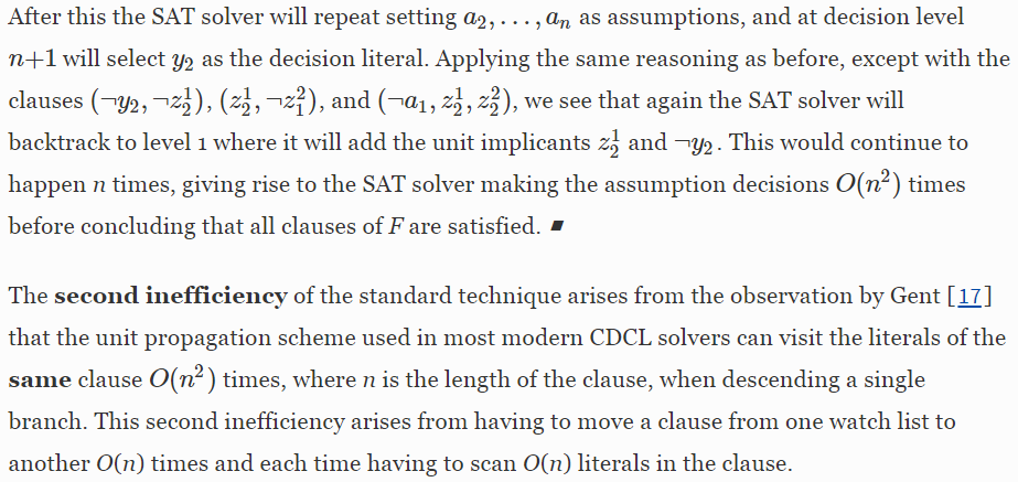
	This backtracking into the various assumption levels to add new implied literals and then having to redo the remaining assumption decisions is the first inefficiency of the standard technique. In some applications, particularly in MaxSat solving, there can often be thousands of assumptions, so this inefficiency can have a significant impact. The following example shows that this inefficiency can potentially induce an overhead that is quadratic in the number of assumptions.
	Example 1
	Example 2
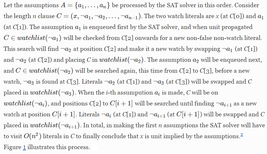
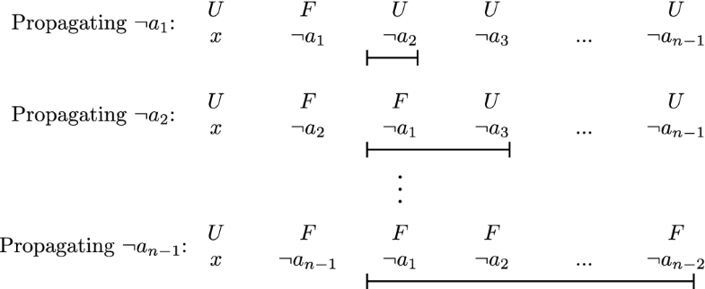
	Fig. 1. The propagate routine searching for a new watcher for clause C of Example 2 when each assumptions is made at a separate decision level and unit propagated before moving to the next assumption. The first two literals are the current watched literals and the line shows the span of literals traversed in searching for a replacement watcher. Truth values are above each literal; “F” represents false, “T” represents true, and “U” represents unassigned.
	3.2 New Approach
	The technique we propose for fixing both of these inefficiencies is very simple. After all literals at level zero have been unit propagated, the SAT solver increments the decision level and enqueues all assumptions at decision level 1, after which it performs unit propagation. So all assumptions are placed on the trail at the top of level 1, and unit propagation is performed only after all assumption literals are on the trail and have been assigned the value truetrue.
	If when processing the assumptions the SAT solver finds one aiai that is already truetrue, then aiai must have been made true at level 0 since unit propagation has not yet been run at level 1. That is, aiai is already on the trail in level 0 and we do not need to enqueue it again so we can skip it. Similarly if aiai is already falsefalse then ¬ai¬ai must have been made true at level 0, so F⊨(¬ai)and the SAT solver can return the conflict clause (¬ai)(¬ai).
	Enqueueing all assumptions at level 1 also necessitates a change to the SAT solver’s analyzeFinal routine which is called in the standard technique to compute a conflict clause when an assumption aiai is about to be enqueued as the i-th decision and is discovered to be falsefalse. We will describe those changes below, but first we explain how our technique fixes the two inefficiencies identified above.
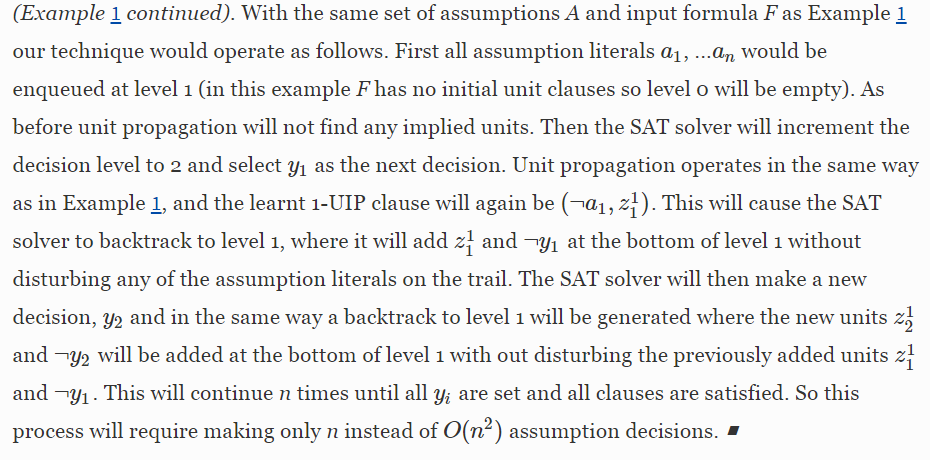
	With our technique all assumptions are at level 1, so if a new unit implicant of the assumptions is found during search, that clause will cause a backtrack to level 1. None of the assignments in level 1 will be undone, instead the new unit will be added to the bottom of level 1 and search will continue after unit propagation is run on the new unit. This resolves the first inefficiency.
	Example 3
	Our technique also addresses the second inefficiency. In particular, since all assumption literals are valued before unit propagation starts, no clause will ever be moved to the watch list of a negated assumption literal as all of these literals are already falsefalse.
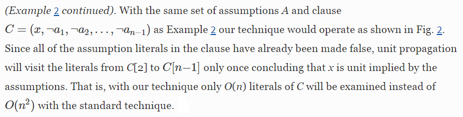
	Fig. 2. The propagate routine searching for a new watcher when all assumptions are enqueued before unit propagation on the clause from Example 2. Line shows span of literals traversed in searching for a replacement watch.
	Example 4
	3.3 Implementation
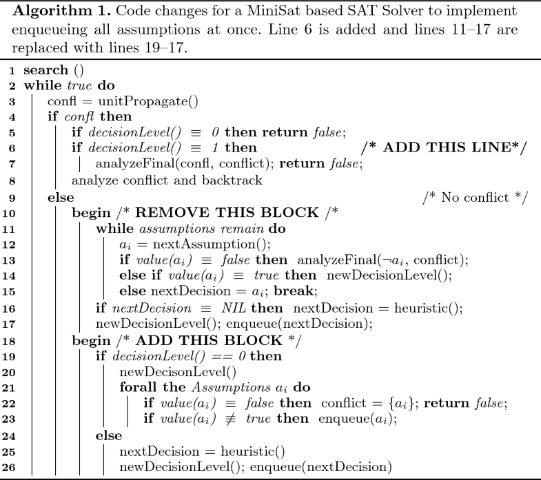
	Our new approach of enqueueing all assumptions at once is very simple to implement, and we illustrate this in the framework of the MiniSat code base. It should be equally easy to implement our approach in non-MiniSat based SAT solvers. Two routines need to be altered: (1) the main search() routine that makes new decisions, invokes unit propagation, and performs clause learning when a conflict is detected; and (2) the analyzeFinal() routine that computes the final conflict clause. The needed changes to the search() routine are shown in Algorithm 1. If a conflict occurs at decision level 1 (where the assumptions are enqueued) we must convert it into a conflict for the assumptions (line 6); and if we are making a decision at level 0 we enqueue all assumptions at level 1 (lines 19–26).
	The routine analyzeFinal() also changes. In the standard approach it is passed an assumption literal that has been falsified by a prior set of assumption decisions (line 13), whereas in the new approach it is passed the conflict clause found at level 1 by unit propagation (line 6). In both cases the routine must return the computed conflict in the passed conflict vector.
	The standard MiniSat implementation starts with C equal to ¬ai¬ai’s reason clause (i.e., the clause that became unit implying ¬ai¬ai). Then while there exists a literal ℓℓ in C not equal to ¬ai¬ai and such that ¬ℓ¬ℓ has been unit implied by reason clause reason(¬ℓ)reason(¬ℓ) we replace C by the resolution of C and reason(¬ℓ)reason(¬ℓ). The end result is a conflict clause that contains ¬ai¬ai and the negation of decision literals. Since, ¬ai¬ai was implied at a level where all decisions are assumptions, the computed clause contains only negated assumption literals as required.
	The new implementation is very similar. It starts with C equal to the passed conflict. Then while there exists a literal ℓℓ in C such that ¬ℓ¬ℓ has been unit implied by reason clause reason(¬ℓ)reason(¬ℓ) we replace C by the resolution of C and reason(¬ℓ)reason(¬ℓ). Since the conflict occurs at level 1 only the assumption literals have no reason clause, so this process removes all non-assumption literals from C and the final result contains only negated assumption literals as required.
	It should be noted however that these two different approaches can produce different conflict clauses even if the initial conflict and trail are similar. In some cases the standard approach might produce a shorter clause and in other cases our new approach might produce a shorter clause.
	Example 5
	The following table illustrates a case where the standard technique will learn a shorter conflict clause.
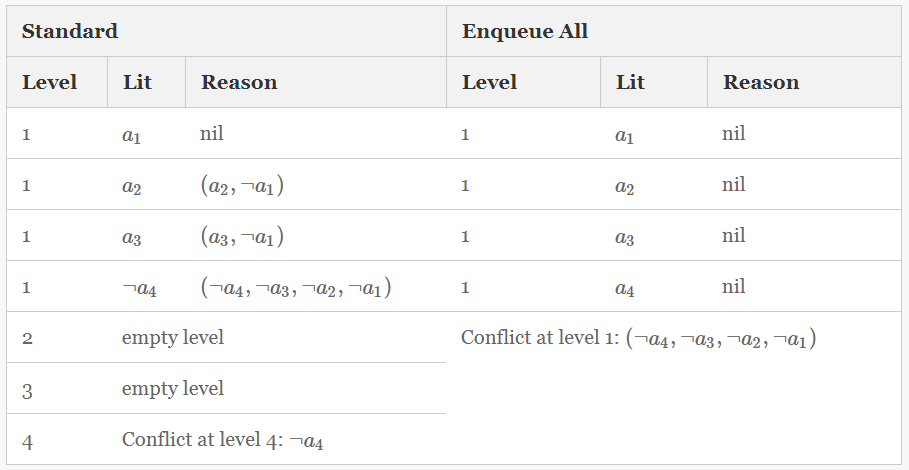
	The table shows the trail when a conflict is found. The left three columns show the trail for the standard approach, and the right three show the trail for our proposed approach of enqueueing all assumptions at level 1. The table indicates the decision level, the literal on the trail and the reason clause. Literals with non-nil reasons are implied literals.
	The standard approach detects a conflict at level 4 when it tries to make a4a4 true as the next decision and finds that a4a4 is already false. The conflict it learns starts with the reason clause for ¬a4¬a4, (¬a4,¬a3,¬a2,¬a1)(¬a4,¬a3,¬a2,¬a1), and proceeds to resolve away all implied literals from this clause except for ¬a4¬a4. This involves resolving away a3a3 and a2a2 to obtain the conflict (¬a4,¬a1)(¬a4,¬a1).
	Our new technique, on the other hand, will enqueue all assumptions at level 1, and then discover that the clause (¬a4,¬a3,¬a2,¬a1)(¬a4,¬a3,¬a2,¬a1) is falsified. In the new technique none of these literals are implied so no resolution steps are performed. Hence it will return this longer clause as the conflict.
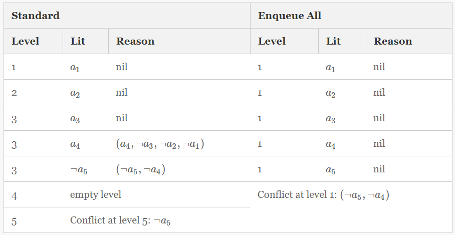
	On the other hand, the following table illustrates a case where the standard technique learns a longer conflict clause.
	The standard technique discovers a conflict at level 5 when it finds that a5a5 is already falsified. Starting with the reason clause (¬a5,¬a4)(¬a5,¬a4), it will resolve away the implied literal ¬a4¬a4 to obtain the conflict clause (¬a5,¬a3,¬a2,¬a1)(¬a5,¬a3,¬a2,¬a1).
	Our new technique, on the other hand, will return the shorter clause (¬a5,¬a4)(¬a5,¬a4) as the conflict, as again none of these literals are implied so no resolution steps will be performed.
	As we will demonstrate later, although our technique could return longer conflicts in the same context, it generally returns shorter ones than the standard technique.
	3.4 Previous Work
	Gent [17] proposed an alternate method for eliminating the second inefficiency where a clause moves from the watch list of one assumption to another many times and each time has many of its literals scanned. In particular, he proposed keeping track of, for each clause, the location where the previous search for a non-falsified literal stopped. Then when a new search is made, the search starts at this previous location and if necessary wraps around. Gent showed that this reduces the worst case number of literals that could be visited in a single clause along a single branch to 2n down from O(n2)O(n2) (n is the clause length). Unlike our approach Gent’s method is more intrusive, requiring a change to the clause data structure (to track the location the previous search stopped). However, it accounts for non-assumption literals as well as assumption literals. Nevertheless, Gent also showed that his technique did not yield any significant gains in SAT solver performance on the instances he experimented with, whereas our technique does yield performance gains, perhaps because it fixes both inefficiencies.
	Audemard et al. [4] proposed four lightweight techniques for improving assumption-based SAT solving in Glucose. First, they ignored the assumption literals when computing the LBD score of a learnt clause. Our method comes close to achieving the same improvement: with it all assumption literals are at the same level, so they contribute only 1 (instead of 0) to the LBD score. Second, they store all of the assumption literals at the end of each learnt clause so as to avoid having to scan these literals on LBD score updates. Third, they check only the two watch literals of a clause to see if it is satisfied to avoid scanning the entire clause.3 Our technique does not achieve the second nor the third improvement.
	Fourth, during unit propagation when scanning a clause for a new non-false watcher, they continue searching until they find a non-false non-assumption literal. If none exist they use the last non-false literal found (even if it is an assumption literal). This technique addresses some of the second inefficiency, but not all of it. In particular, if in Example 2 the assumptions A are set in the order a1a1, an−1an−1, an−2an−2, ..., a2a2 then the clause (x,¬a1,¬a2,…,¬an−1)(x,¬a1,¬a2,…,¬an−1) will still have its literals scanned O(n2)O(n2) times when each assumption is a separate decision. For example, when a1a1 is made true, all of the literals ¬a2¬a2, ..., ¬an−1¬an−1 will be scanned, skipping over non-false assumption literals, until finally returning the last non-false assumption literal ¬an−1¬an−1 as the new watcher.
	It can also be noted that none of the techniques of [4, 17] address the first inefficiency.

 

 

 

4 Trail Savings

	When a restart returns the SAT solver to level zero, the solver can often proceed to reproduce the same initial sequence of decisions that were on the trail before the restart. Redoing these decisions is redundant work and methods for saving this work by making the SAT solver backtrack only to the point where the restart causes a divergence in the decisions made have been developed [31]. Similarly, [4] proposes only backtracking to the bottom of the assumption levels on restart, as all of the assumption decisions will be redone by the solver.
	However, these techniques do not help when the SAT solver learns a new unit clause. Unit clauses are added to level 0 so the solver must backtrack across the assumptions to insert the new unit into the trail. After this it must redo the assumptions. Our trail savings method is based on the observation that after a new unit is added to level 0, the set of literals forced to be true at level 0 and 1 can only either (a) be contradictory or (b) be a superset of the previous set of literals forced at level 0 and 1.
	Our new technique based on this observation is as follows. When a new unit is learnt we save a copy of the level 1 trail (all literals and clause reasons). Then we backtrack the trail to the end of level 0, add the new unit, and perform unit propagation. If no contradiction is found we then enqueue each literal from our copy of the level 1 preserving the order these literals previously appeared on the trail (so assumptions are enqueued first). If any of these literals is already truetrue, we skip enqueueing it. If any of these literals is already falsefalse, we can compute a conflict for the assumptions. If the falsified literal is an assumption ¬ai¬ai then the conflict is (¬ai)(¬ai), otherwise the conflict is computed by passing the stored reason clause associated with the falsified literal (this reason clause has become falsified at level 1) to analyzeFinal to compute the conflict. After all saved literals have been added to level 1, we invoke unit propagation from the top of level 1. Note that although we can restore the literals from level 1 we still have to unit propagate them once again. However, this unit propagation process is sped up by the fact that many literals have already been made truetrue at level 1. Hence, the second inefficiency of moving a clause from one watch literal to another will occur less frequently.
	We can further extend trail savings to provide a head start for the SAT solver when it is called again with a different set of assumptions. Note that level 0 is always preserved between calls to the SAT solver as this level does not depend on the assumptions. Our extension is to also try to preserve as much of level 1 as is possible between SAT calls. The method is to save all of the literals implied at level 1, and their reason clauses, at the time the SAT solver exits. Then when the SAT solver is called again with a new set of assumptions, we enqueue all of these assumptions at level 1 as normal. After the new assumptions are enqueued, and before they are unit propagated, we check all of the saved literals previously implied at level 1, in the order they were previously on the trail. If their reasons are still unit clauses under the new trail, we enqueue them on the trail with the same reason clause.4 Note that by examining these implied literals in trail order we can detect preserved implied literals that rely on previously preserved implied literals. For example, say x and y were at level 1 at the end of the previous SAT solve with y appearing after x, and with reason clauses (x,¬a1)(x,¬a1) and (y,¬x)(y,¬x). Then if the new SAT call includes the previous assumption a1a1 our technique will detect that x is still unit implied with the same reason clause, and x will be added to the trail. Then y will also be detected to still be unit because x has already been added to the trail.

 

5 Experiments and Results

	We implemented our techniques in the MiniSat 2.2 and Glucose 3.0 SAT solvers. In Glucose 3.0 we also preserved the already implemented incremental techniques of [4]. We then used these modified SAT solvers in the MaxHS [12] and RC2 [18] MaxSat solvers, both of which are state-of-the-art MaxSat solvers. MaxHS uses MiniSat while RC2 uses Glucose.
	We then ran these solvers using both the modified and original SAT solvers on 7439 benchmark instances (4627 unweighted and 2812 weighted) collected from the 2008 to 2018 MaxSat Evaluations [1]. This benchmark set includes all non-random instances used and submitted to these evaluations, excluding 825 “abrame-habet” random maxcut instances that were categorized as “crafted” instances (none of these are solvable by either MaxHS nor RC2). We also removed duplicate instances that had different names but were the same except for comment lines. The experiments were run on 2.4 GHz Intel cores with 30 min CPU time and 5.24 GB memory limits.
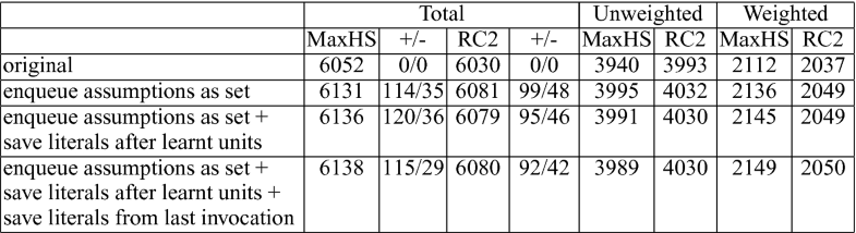
	Fig. 3. Number of MaxSat instances solved by MaxHS and RC2 using different extensions of the underlying SAT solver. The +/− column shows the number of instances gained/lost vs the original.
	Figure 3 shows that our first technique of enqueueing all assumptions at once is surprisingly effective yielding 79 newly solved instances for MaxHS and 51 newly solved instances for RC2. It should be noted that both of these solvers are state-of-the-art and techniques that allow them to solve this many new instances are not easy to find. Trail savings within the same SAT solver call is a less successful improvement. It gains 5 more problems for MaxHS but loses 2 problems for RC2. Trail savings across different SAT solver calls, is even less impactful. Hence, in terms of number of instances solved trail savings do not seem to be either positively or negatively significant, and the remaining experiments use only the enqueueing technique.
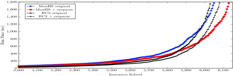
	Fig. 4. Cactus plot comparing total instances solved within a given time bound for MaxHS and RC2 with and without our assumption enqueueing techniques. The first 5000 instances were solved in less than 50 s each, so that part of the plot is truncated.
	Figure 4 shows a cactus plot of the two solvers with and without enqueueing. The plot shows that enqueueing provides a general speedup for both solvers with more instances generally being solved at every time bound in the plot. Note the first 5000 instances were solved by both solvers in ≤≤50 s per instance, so we truncated that part of the plot to show more detail on the harder instances.
	The run times shown in Fig. 4 are affected both by the speed of the SAT solver and by the sequence of conflicts returned by the different SAT solvers. That is, the SAT calls the MaxSat solver performs diverges as the instance is solved. Hence, to get a more precise picture of the SAT solver speedup and the quality of conflicts obtained by our technique, we changed RC2 so that it always invokes both the original Glucose solver and then the modified Glucose solver with enqueueing. However, RC2 always uses the conflict returned by the original Glucose solver in its further processing. In this way, each version of the SAT solver is solving an identical sequence of SAT calls during the processing of each MaxSat instance. We ran this modified version of RC2 on the same suite of 7439 MaxSat instances, giving it 3600 s per instance to account for the doubled up SAT solving. From this setup we obtained a sequence of matched pairs of SAT solver calls where the standard and equeueing versions of the SAT solver are both invoked to solve the same formula subject to the same set of assumptions and with the same history of previous calls.
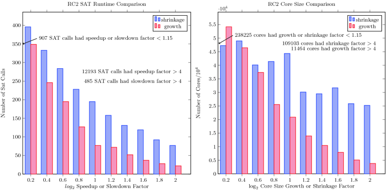
	We measured the CPU time each SAT solver call took in each matched pair, discarding those pairs where both solvers took less than 0.1 s. In particular, we did not compare the CPU times of SAT solver calls that were so fast that they were likely to be too noisy. This yielded 22,810 matched pairs of SAT solver calls. There is quite a bit of variance in the runtimes, so a scatter plot of these points was not very informative. Instead for each pair we computed log2( Original  Glucose  CPU  Enqueueing  Glucose  CPU )log2⁡( Original  Glucose  CPU  Enqueueing  Glucose  CPU ). This number is positive when original Glucose is slower and symmetric but negative when original Glucose is faster. Hence, the absolute value of the negative numbers represent instances that had that log2log2 speedup ratio, while the positive numbers represent instances that had that log2log2 slowdown ratio. Figure 5 left shows a side-by-side histogram of the number of instances that had similar amounts of log2log2 speedup and slowdown ratio. The Figure shows that although there is considerable variance among the instances—some were sped up while others were slowed down—there is a general trend that for all bands of speedup/slowdown factors more instances had a speedup of that factor than had a slowdown of that factor.
	Fig. 5. Left: Comparison of number of instances that had corresponding log2log2 speedups or slowdowns. Right: Individual core size (right) log2log2 comparison.
	We measured the CPU time each SAT solver call took in each matched pair, discarding those pairs where both solvers took less than 0.1 s. In particular, we did not compare the CPU times of SAT solver calls that were so fast that they were likely to be too noisy. This yielded 22,810 matched pairs of SAT solver calls. There is quite a bit of variance in the runtimes, so a scatter plot of these points was not very informative. Instead for each pair we computed     growth and shrinkage ratios: shrinkage indicates that enqueueing Glucose produces a shorter conflict, while growth indicates that it produces a longer conflict. As with the run times there is a considerable variance in core sizes among these identical SAT calls—on some calls enqueueing Glucose produced larger conflicts, and on others it produced smaller conflicts. Nevertheless, the general trend is that for any band of growth/shrinkage ratio, more conflicts produced by enqueueing Glucose had that amount of shrinkage than that amount of growth. The only divergence from this trend was that there were more cores grown by a log2log2 factor between 0.1 to 0.3 (the band centered at 0.2) than shrunk by this factor. Most notably, however, almost 10 times as many cores were more than a factor of 4 smaller than were more than a factor of 4 larger.
	This experiment shows that the overall better performance of enqueueing Glucose in RC2 is likely a product of both faster SAT calls and smaller conflicts. Together these two effects tend to make RC2 more effective. Although we do not have similar data for MiniSat used in MaxHS, we expect that similar results hold since MaxHS is also more effective with enqueueing.
	Although we do not have space to show the data, we also experimented with MUS extraction in the Muser tool [8], and showed that our techniques speed up Muser and allowed it to produce smaller MUSes. In the benchmark suite we used for Muser we were not able, however, to solve any additional instances. The heavier-weight techniques of [19] (involving introducing new abbreviation literals) were able solve additional instances mainly by reducing Muser’s memory footprint. Similarly, although the data presented above about number of instances solved does not convincingly demonstrate the effectiveness of our proposed trail saving techniques, finer grained data does indicate that these ideas do tend to yield run time speedups.

6 Conclusion

We have introduced some simple ideas for improving the efficiency of assumption-based SAT solving. Or experiments show that the easiest of these to implement, enqueueing all assumptions at level 1, is quite effective in improving MaxSat solvers. For future work, Example 5 indicates that finding a way to combine clause minimization with our enqueueing technique might yield shorter conflicts. Furthermore, finding ways of exploiting our trail savings technique at levels besides level 1 might make this idea more useful.

 

Footnotes

1. Quick checks to determine if C is already satisfied can be made first by checking data in the watch data structure (the blocking literal) and checking if the clause’s other watch is truetrue.

2. 2.

   This description follows the MiniSat and Glucose schemes for watch literals, but this particular type of implementation is not necessary. Scanning O(n2)O(n2) literals in the clause down a single branch occurs with any implementation that stores no information about the previous scan [17].

3. 3.

   It is not clear if this third technique is an improvement outside of the context of MUS extraction.

4. 4.

   We save a reference to the reason clause, so before checking to see if the reason is still unit we must ensure that the references haven’t been changed by garbage collection, and that the implied literal is still at position zero in the reason clause (this is a MiniSat invariant for reason clauses).

References

1. 1.
   Maxsat evaluation series: 2006–2016 http://www.maxsat.udl.cat/, 2017–2018 https://maxsat-evaluations.github.io/
2. 2.
   Alviano, M., Dodaro, C., Ricca, F.: A MaxSat algorithm using cardinality constraints of bounded size. In: Proceedings of the Twenty-Fourth International Joint Conference on Artificial Intelligence, IJCAI 2015, Buenos Aires, Argentina, 25–31 July 2015, pp. 2677–2683 (2015). http://ijcai.org/Abstract/15/379
3. 3.
   Ansótegui, C., Didier, F., Gabàs, J.: Exploiting the structure of unsatisfiable cores in MaxSat. In: Proceedings of the Twenty-Fourth International Joint Conference on Artificial Intelligence, IJCAI 2015, Buenos Aires, Argentina, 25–31 July 2015, pp. 283–289 (2015). http://ijcai.org/Abstract/15/046
4. 4.
   Audemard, G., Lagniez, J.-M., Simon, L.: Improving glucose for incremental SAT solving with assumptions: application to MUS extraction. In: Järvisalo, M., Van Gelder, A. (eds.) SAT 2013. LNCS, vol. 7962, pp. 309–317. Springer, Heidelberg (2013).  https://doi.org/10.1007/978-3-642-39071-5_23CrossRefzbMATHGoogle Scholar
5. 5.
   Bacchus, F., Davies, J., Tsimpoukelli, M., Katsirelos, G.: Relaxation search: a simple way of managing optional clauses. In: Proceedings of the Twenty-Eighth AAAI Conference on Artificial Intelligence, 27–31 July 2014, Québec City, Québec, Canada, pp. 835–841 (2014). http://www.aaai.org/ocs/index.php/AAAI/AAAI14/paper/view/8618
6. 6.
   Bacchus, F., Katsirelos, G.: Using minimal correction sets to more efficiently compute minimal unsatisfiable sets. In: Kroening, D., Păsăreanu, C.S. (eds.) CAV 2015. LNCS, vol. 9207, pp. 70–86. Springer, Cham (2015).  https://doi.org/10.1007/978-3-319-21668-3_5CrossRefGoogle Scholar
7. 7.
   Belov, A., Lynce, I., Marques-Silva, J.: Towards efficient MUS extraction. AI Commun. 25(2), 97–116 (2012).  https://doi.org/10.3233/AIC-2012-0523MathSciNetCrossRefzbMATHGoogle Scholar
8. 8.
   Belov, A., Marques-Silva, J.: Muser2: an efficient MUS extractor. JSAT 8(3/4), 123–128 (2012). https://satassociation.org/jsat/index.php/jsat/article/view/101zbMATHGoogle Scholar
9. 9.
   Biere, A.: Cadical, Lingeling, Plingeling, Treengeling and YalSAT entering the sat competition 2018. In: Heule, M.J.H., Järvisalo, M., Suda, M. (eds.) Proceedings of SAT COMPETITION 2018 Solver and Benchmark Descriptions. University of Helsinki (2018)Google Scholar
10. 10.
    Cabodi, G., Lavagno, L., Murciano, M., Kondratyev, A., Watanabe, Y.: Speeding-up heuristic allocation, scheduling and binding with sat-based abstraction/refinement techniques. ACM Trans. Design Autom. Electr. Syst. 15(2), 121–1234 (2010).  https://doi.org/10.1145/1698759.1698762CrossRefGoogle Scholar
11. 11.
    Claessen, K., Sörensson, N.: A liveness checking algorithm that counts. In: Formal Methods in Computer-Aided Design, FMCAD 2012, Cambridge, UK, 22–25 October 2012, pp. 52–59 (2012). http://ieeexplore.ieee.org/document/6462555/
12. 12.
    Davies, J., Bacchus, F.: Solving MAXSAT by solving a sequence of simpler SAT instances. In: Proceedings Principles and Practice of Constraint Programming - CP 2011–17th International Conference, CP 2011, Perugia, Italy, 12–16 September 2011, pp. 225–239 (2011). https://doi.org/10.1007/978-3-642-23786-7_19CrossRefGoogle Scholar
13. 13.
    Davies, J., Bacchus, F.: Postponing optimization to speed up MAXSAT solving. In: Proceedings of the Principles and Practice of Constraint Programming - 19th International Conference, CP 2013, Uppsala, Sweden, 16–20 September 2013, pp. 247–262 (2013). https://doi.org/10.1007/978-3-642-40627-0_21Google Scholar
14. 14.
    Eén, N., Mishchenko, A., Amla, N.: A single-instance incremental SAT formulation of proof- and counterexample-based abstraction. In: Proceedings of 10th International Conference on Formal Methods in Computer-Aided Design, FMCAD 2010, Lugano, Switzerland, 20–23 October, pp. 181–188 (2010).http://ieeexplore.ieee.org/document/5770948/
15. 15.
    Eén, N., Sörensson, N.: An extensible SAT-solver. In: Giunchiglia, E., Tacchella, A. (eds.) SAT 2003. LNCS, vol. 2919, pp. 502–518. Springer, Heidelberg (2004).  https://doi.org/10.1007/978-3-540-24605-3_37CrossRefGoogle Scholar
16. 16.
    Eén, N., Sörensson, N.: Temporal induction by incremental SAT solving. Electr. Notes Theor. Comput. Sci. 89(4), 543–560 (2003).  https://doi.org/10.1016/S1571-0661(05)82542-3CrossRefzbMATHGoogle Scholar
17. 17.
    Gent, I.P.: Optimal implementation of watched literals and more general techniques. J. Artif. Intell. Res. 48, 231–251 (2013).  https://doi.org/10.1613/jair.4016MathSciNetCrossRefzbMATHGoogle Scholar
18. 18.
    Ignatiev, A., Morgado, A., Marques-Silva, J.: RC2: a python-based MaxSat solver. In: Bacchus, F., Järvisalo, M., Martins, R. (eds.) MaxSAT Evaluation 2018 Solver and Benchmark Descriptions. University of Helsinki (2018)Google Scholar
19. 19.
    Lagniez, J.-M., Biere, A.: Factoring out assumptions to speed up MUS extraction. In: Järvisalo, M., Van Gelder, A. (eds.) SAT 2013. LNCS, vol. 7962, pp. 276–292. Springer, Heidelberg (2013).  https://doi.org/10.1007/978-3-642-39071-5_21CrossRefGoogle Scholar
20. 20.
    Liffiton, M.H., Previti, A., Malik, A., Marques-Silva, J.: Fast, flexible MUS enumeration. Constraints 21(2), 223–250 (2016).  https://doi.org/10.1007/s10601-015-9183-0MathSciNetCrossRefzbMATHGoogle Scholar
21. 21.
    Martins, R., Manquinho, V., Lynce, I.: Open-WBO: a modular MaxSAT solver,. In: Sinz, C., Egly, U. (eds.) SAT 2014. LNCS, vol. 8561, pp. 438–445. Springer, Cham (2014).  https://doi.org/10.1007/978-3-319-09284-3_33CrossRefGoogle Scholar
22. 22.
    Mencía, C., Previti, A., Marques-Silva, J.: Literal-based MCS extraction. In: Proceedings of the Twenty-Fourth International Joint Conference on Artificial Intelligence, IJCAI 2015, Buenos Aires, Argentina, 25–31 July 2015, pp. 1973–1979 (2015). http://ijcai.org/Abstract/15/280
23. 23.
    Morgado, A., Dodaro, C., Marques-Silva, J.: Core-guided MaxSAT with soft cardinality constraints. In: Proceedings of the Principles and Practice of Constraint Programming - 20th International Conference, CP 2014, Lyon, France, 8–12 September 2014, pp. 564–573 (2014). https://doi.org/10.1007/978-3-319-10428-7_41Google Scholar
24. 24.
    Nadel, A., Ryvchin, V.: Efficient SAT Solving under assumptions. In: Cimatti, A., Sebastiani, R. (eds.) SAT 2012. LNCS, vol. 7317, pp. 242–255. Springer, Heidelberg (2012).  https://doi.org/10.1007/978-3-642-31612-8_19CrossRefzbMATHGoogle Scholar
25. 25.
    Nadel, A., Ryvchin, V., Strichman, O.: Ultimately incremental SAT. In: Sinz, C., Egly, U. (eds.) SAT 2014. LNCS, vol. 8561, pp. 206–218. Springer, Cham (2014).  https://doi.org/10.1007/978-3-319-09284-3_16CrossRefzbMATHGoogle Scholar
26. 26.
    Narodytska, N., Bacchus, F.: Maximum satisfiability using core-guided MaxSat resolution. In: Proceedings of the Twenty-Eighth AAAI Conference on Artificial Intelligence, Québec City, Québec, Canada, 27–31 July 2014, pp. 2717–2723 (2014). http://www.aaai.org/ocs/index.php/AAAI/AAAI14/paper/view/8513
27. 27.
    Previti, A., Mencía, C., Järvisalo, M., Marques-Silva, J.: Improving MCS enumeration via caching. In: Proceedings of the Theory and Applications of Satisfiability Testing - SAT 2017–20th International Conference, Melbourne, VIC, Australia, 28 August–1 September 2017, pp. 184–194 (2017).  https://doi.org/10.1007/978-3-319-66263-3_12CrossRefGoogle Scholar
28. 28.
    Saikko, P., Berg, J., Järvisalo, M.: LMHS: A SAT-IP hybrid MaxSAT solver. In: Creignou, N., Le Berre, D. (eds.) SAT 2016. LNCS, vol. 9710, pp. 539–546. Springer, Cham (2016).  https://doi.org/10.1007/978-3-319-40970-2_34CrossRefzbMATHGoogle Scholar
29. 29.
    Silva, J.P.M., Lynce, I., Malik, S.: Conflict-driven clause learning SAT solvers. In: Handbook of Satisfiability, pp. 131–153. IOS Press (2009). https://doi.org/10.3233/978-1-58603-929-5-131
30. 30.
    Soos, M.: The cryptominisat 5.5 set of solvers at the sat competition 2018. In: Heule, M.J.H., Järvisalo, M., Suda, M. (eds.) Proceedings of SAT COMPETITION 2018 Solver and Benchmark Descriptions. University of Helsinki (2018)Google Scholar
31. 31.
    van der Tak, P., Ramos, A., Heule, M.: Reusing the assignment trail in CDCL solvers. JSAT 7(4), 133–138 (2011). https://satassociation.org/jsat/index.php/jsat/article/view/89MathSciNetzbMATHGoogle Scholar