
机器学习编程01_线性回归
machine-learning-01 线性回归模拟
跟随吴恩达老师学习机器学习,利用Octave开源软件,快速实现模型建立与函数实现,开启了我在机器学习领域的大门。今天是机器学习的第一个编程作业——线性回归。希望和大家一起学习,共同进步。
I.Simple Octave function:返回5*5的矩阵
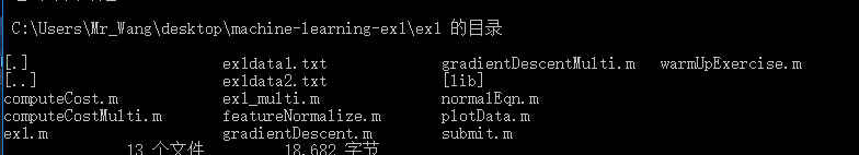
1.下载好ex1文件并load到Octave中
2.编写warmUpExercise.m文件
function A = warmUpExercise()
%WARMUPEXERCISE Example function in octave
%   A = WARMUPEXERCISE() is an example function that returns the 5x5
%  identity matrix
A = eye(5);
% ============= YOUR CODE HERE ==============
% Instructions: Return the 5x5 identity matrix
%               In octave, we return values by defining which variables
%               represent the return values (at the top of the file)
%               and then set them accordingly.
% ===========================================
end
3.在Octave中运行warmwarmUpExercise函数

II.Linear regression with one variable
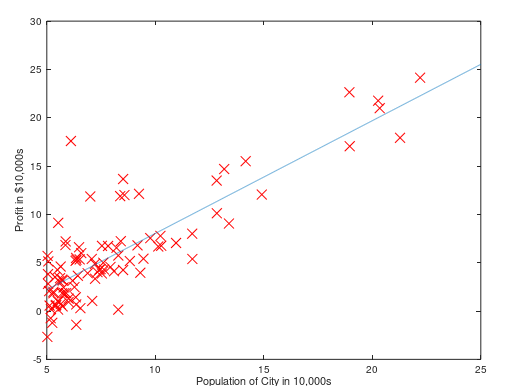
单特征值的线性回归预测,ex1data1中包含了97组数据,每组有两个数据用“,”分割,一个为x变量,一个为y因变量。
1.将数据load到Octave中 & 编写plotData.m文件
data = load('ex1data1.txt'); % read comma separated data
X = data(:, 1); y = data(:, 2);
m = length(y); % number of training examples
function plotData(x, y)
plot(x, y, 'bx', 'MarkerSize', 10); % Plot the data
ylabel('Profit in $10,000s'); % Set the y?axis label
xlabel('Population of City in 10,000s');

end
2.运行poltData函数

3.Gradient Descent
%初始值设定
X = [ones(m, 1), data(:,1)]; % Add a column of ones to x
theta = zeros(2, 1); % initialize fitting parameters
iterations = 1500;
alpha = 0.01;
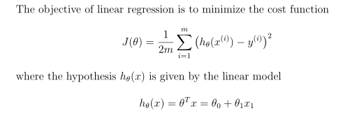
%computeCost函数编写
function J = computeCost(X, y, theta)
m = length(y); % number of training examples
J = sum(power(X*theta-y,2)/(2*m));
end
运行得到期望值32.07

%计算theta_0,theta_1 & 编写gradientDescent函数
%num_iters    --->   iterations
function [theta, J_history] = gradientDescent(X, y, theta, alpha, num_iters)
m = length(y); % number of training examples
J_history = zeros(num_iters, 1);

for iter = 1:num_iters
    theta1=theta(1,1)-alpha/m*sum(X*theta-y);
    theta2=theta(2,1)-alpha/m*sum((X*theta-y) .* X(:,2));
    theta(1,1)=theta1;
    theta(2,1)=theta2;
J_history(iter) = computeCost(X, y, theta);

end
end
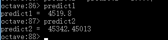
计算预测值
predict1 = [1, 3.5]theta;
predict2 = [1, 7]theta;
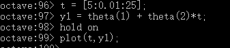
4.通过gradientDescent求出的theta值画出拟合曲线
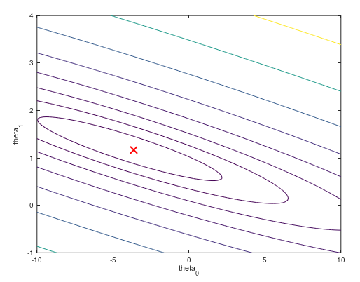
III.Visualizing->understand better gradientDescent function
将数据与回归直线的误差J转化为三维像小山一样的模型,我们通过梯度下降算法找到极小值点,利用等高线图像,在凹线中心的地方为最好的拟合点,更好的理解梯度下降算法的原理。
%初始化变量
% Grid over which we will calculate J
theta0_vals = linspace(-10, 10, 100);
theta1_vals = linspace(-1, 4, 100);

% initialize J_vals to a matrix of 0's
J_vals = zeros(length(theta0_vals), length(theta1_vals));

% Fill out J_vals
for i = 1:length(theta0_vals)
    for j = 1:length(theta1_vals)
	  t = [theta0_vals(i); theta1_vals(j)];
	  J_vals(i,j) = computeCost(X, y, t);
    end
end
%3-d误差模型
figure;
surf(theta0_vals, theta1_vals, J_vals)

%误差等高线模型
figure
contour(theta0_vals, theta1_vals, J_vals, logspace(-2, 3, 20)) %画20条等高线,每条等高线的值根据theta0,theta1,J,在10^(-2)和10^3依次对应一个值

hold on;
plot(theta(1), theta(2), 'rx', 'MarkerSize', 10, 'LineWidth', 2);
笔者能力有限,哪里理解的不好请大家不要吝啬指出,不胜感激。

 浙公网安备 33010602011771号