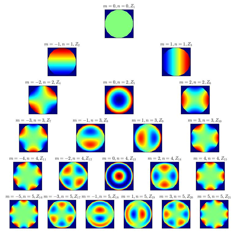
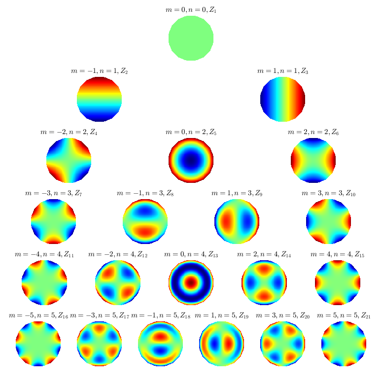
MATLAB绘制前21个Zernike多项式,按照径向级次$n$垂直排序,角向级次$m$水平排序
背景知识
我们直观地将各种成像缺陷分为一系列的像差,如倾斜、球差、彗差、场屈、象散、畸变等。
\(\lambda\)是波长
波矢量是矢量,波数是标量,波矢量的大小称为波数。波数\(k\)表示什么含义?单位传播距离相位变化量,公式是\(k=2\pi/\lambda\)
波前\(\Phi\)定义为传播路径的长度(常以波长为单位),而相位\(S\)正比于传播路径的长度与波长的比值,二者的关系为:
\(S=2\pi \Phi /\lambda =k \Phi\)
一般采用波前(等相位面,wave front)来描述像差。一种广泛使用的方法是将实际光波的复杂波前表示为 一系列的正交多项式的组合,最常用的是Zernike多项式。Zernike多项式是在圆域上对径向变量和角度变量的连续函数正交的二维多项式,一般表示成极坐标\((\theta,\rho)\)的形式,\(\rho\)为单位径向坐标,\(\theta\)为极角坐标。
在各种文献中,Zernike多项式的形式略有差别,较易引起混乱。
结果
代码
原版,我一开始写的,每个subplot有边框
clear all;close all;clc;
% Define the range for n and m
n_values = 0:5;
pixels=100;%image x,y pixels

%%The transverse and longitudinal dimensions of the pupil surface
% can enhance the Fourier transform results by reducing the proportion of pupil area
q=300;


% Initialize a figure
fig=figure('name','ZernikePolynomials');
figWidth = 620; % Set the figure width
figHeight = 620; % Set the figure height
set(fig, 'Position', [200, 200, figWidth, figHeight]);


%% Creating mask for unit circle
X = linspace(-1, 1, pixels);
[X, Y] = meshgrid(X, X);
circleMask = (X.^2 + Y.^2) <= 1;


% Loop over n values
for i = 1:length(n_values)
    n = n_values(i);

    % Loop over m values, incrementing by 2
    for m = -n:2:n
        % Calculate index for the subplot
        subplot_index = (i-1)*(n+1) + (m+n)/2 + 1;

        % Calculate radial polynomial
        [RmnC,rhoExp] = calcRmn(abs(m),n);
        % Calculate zernike polynomial as raster scan
        myData = zeros(pixels);
        myData = calcZP(RmnC,rhoExp,m,n,pixels);

        % Apply mask to myData
        myData(~circleMask) = NaN;


        % Create subplot
        margin=0.04; % Adjust this to control the spacing between subplots
        subplot_tight(length(n_values), n+1, subplot_index, margin);
        imagesc(myData);
        axis square;
        colormap("jet");
        title(['$m=' num2str(m) ', n=' num2str(n) ', Z_{' num2str(subplot_index-(1+n)*n/2 ) '}$'], 'Interpreter', 'latex');

        % Remove x and y labels
        set(gca,'xtick',[],'ytick',[]);
    end
end


%%
function [PC,PExp]=calcRmn (m,n)
%CALCRMN calculate the radial polynomial
%Inputs Zernike polynomial values m,n
%Returns the coefficients for polynomial exponents
%Parameters
OET=(n-m);%check if odd or even
mC=OET/2;%number of coefficients calculated
%Initialize
RmnC= zeros(1,mC);
rhoExp=zeros(1,mC);
%Calculation of radial polynomial
if mod(OET,2)==0
    %do if test is even;otherwise dont
    k=0;Rmn=0;
    while k<=mC
        Rmn=(-1)^k*factorial(n-k)/(factorial(k)*factorial((n+m)/2-k)*factorial((n-m)/2-k));
        k=k+1;
        PC(k)=Rmn;%Polynomial coefficients
        PExp(k)=(n-2*(k-1));%Polynomial exponents
    end
end
end%End function

function mD =calcZP(RmnC,rhoExp,m,n,pX)
%CALCZP calculate the zernike polynomial shape
%Inputs radial polynomial,plus m,n,pixels
%Returns the Zernike polynomial data set
%Calculate Zernike polynomial shape
mD=zeros(pX);
for r=1:pX
    for c=1:pX
        x=(2*c-pX-1)/pX;%convert to x,y
        y=(2*r-pX-1)/pX;%convert to x,y
        %Calculate quadrant correct angle
        phi=atan2(y,x);
        %Convert rectangular coord to distance
        rho=sqrt(x^2+y^2);
        RMN =0;
        for count =1:(n-abs(m))/2+1
            RMN =RMN+RmnC(count)*rho.^rhoExp(count);
        end
        %Calculate ZP wavefront
        if m<0 || n==0   %select for+/-m
            Z=-RMN*sin(abs(m)*phi);
        else
            Z=RMN*cos(abs(m)*phi);
        end
        %Control visual appearance
        if rho<=1%zero outside unit circle
            mD(r,c)=Z;%load value
        else
            mD(r,c)=0;%change to Nan to hide
        end
    end
end
end%End Function
修订版,每个subplot无边框,圆形外区域直接设置为白色
clear all;close all;clc;
% Define the range for n and m
n_values = 0:5;
pixels=100;%image x,y pixels

%%The transverse and longitudinal dimensions of the pupil surface
% can enhance the Fourier transform results by reducing the proportion of pupil area
q=300;


% Initialize a figure
fig=figure('name','ZernikePolynomials', 'Color', [1 1 1]); % 将当前图形背景色设置为白色
figWidth = 620; % Set the figure width
figHeight = 620; % Set the figure height
set(fig, 'Position', [200, 200, figWidth, figHeight]);


%% Creating mask for unit circle
X = linspace(-1, 1, pixels);
[X, Y] = meshgrid(X, X);
circleMask = (X.^2 + Y.^2) <= 1;


% Loop over n values
for i = 1:length(n_values)
    n = n_values(i);

    % Loop over m values, incrementing by 2
    for m = -n:2:n
        % Calculate index for the subplot
        subplot_index = (i-1)*(n+1) + (m+n)/2 + 1;

        % Calculate radial polynomial
        [RmnC,rhoExp] = calcRmn(abs(m),n);
        % Calculate zernike polynomial as raster scan
        myData = zeros(pixels);
        myData = calcZP(RmnC,rhoExp,m,n,pixels);

        % Apply mask to myData
        myData(~circleMask) = NaN;


        %         % Create subplot
        %         margin=0.04; % Adjust this to control the spacing between subplots
        %         subplot_tight(length(n_values), n+1, subplot_index, margin);
        %         imagesc(myData);
        %         axis square;
        %         colormap("jet");
        %         title(['$m=' num2str(m) ', n=' num2str(n) ', Z_{' num2str(subplot_index-(1+n)*n/2 ) '}$'], 'Interpreter', 'latex');
        %
        %         % Remove x and y labels
        %         set(gca,'xtick',[],'ytick',[]);
        % Create subplot
        margin=0.04; % Adjust this to control the spacing between subplots
        subplot_tight(length(n_values), n+1, subplot_index, margin);

        % Set the background color for areas outside the unit circle
        %         backgroundColorValue = min(myData(:)) - 1; % Assuming that the background is the highest value plus 1.
        backgroundColorValue = NaN; % Assuming that the background is the highest value plus 1.
        myData(~circleMask) = backgroundColorValue;


        my_image=imagesc(myData);
        %         imagesc(myData, [min(myData(:)) max(myData(:))] );
        box off;
        axis square;
        % jet, hot, autumn, parula, hsv, cool, spring, summer, winter,
        % gray, bone, copper, pink,  lines, colorcube, prism, flag, white
        colormap([ jet(1024) ]); % Append the background color to the current colormap
        set(my_image, 'AlphaData', ~isnan(myData));
        %         colormap([ jet(2048) ]); % Append the background color to the current colormap
        title(['$m=' num2str(m) ', n=' num2str(n) ', Z_{' num2str(subplot_index-(1+n)*n/2 ) '}$'], 'Interpreter', 'latex');

        % Remove x and y labels
        %         set(gca,'xtick',[],'ytick',[]);
        %         set(gca, 'Visible', 'off');
        % 获取当前坐标轴
        ax = gca;

        % 关闭边框框线
        ax.Box = 'off';

        % 隐藏坐标轴刻度标签
        ax.XAxis.TickLabels = {};
        ax.YAxis.TickLabels = {};

        % 隐藏坐标轴线条
        ax.XAxis.Visible = 'off';
        ax.YAxis.Visible = 'off';

    end
end


%%
function [PC,PExp]=calcRmn (m,n)
%CALCRMN calculate the radial polynomial
%Inputs Zernike polynomial values m,n
%Returns the coefficients for polynomial exponents
%Parameters
OET=(n-m);%check if odd or even
mC=OET/2;%number of coefficients calculated
%Initialize
RmnC= zeros(1,mC);
rhoExp=zeros(1,mC);
%Calculation of radial polynomial
if mod(OET,2)==0
    %do if test is even;otherwise dont
    k=0;Rmn=0;
    while k<=mC
        Rmn=(-1)^k*factorial(n-k)/(factorial(k)*factorial((n+m)/2-k)*factorial((n-m)/2-k));
        k=k+1;
        PC(k)=Rmn;%Polynomial coefficients
        PExp(k)=(n-2*(k-1));%Polynomial exponents
    end
end
end%End function

function mD =calcZP(RmnC,rhoExp,m,n,pX)
%CALCZP calculate the zernike polynomial shape
%Inputs radial polynomial,plus m,n,pixels
%Returns the Zernike polynomial data set
%Calculate Zernike polynomial shape
mD=zeros(pX);
for r=1:pX
    for c=1:pX
        x=(2*c-pX-1)/pX;%convert to x,y
        y=(2*r-pX-1)/pX;%convert to x,y
        %Calculate quadrant correct angle
        phi=atan2(y,x);
        %Convert rectangular coord to distance
        rho=sqrt(x^2+y^2);
        RMN =0;
        for count =1:(n-abs(m))/2+1
            RMN =RMN+RmnC(count)*rho.^rhoExp(count);
        end
        %Calculate ZP wavefront
        if m<0 || n==0   %select for+/-m
            Z=-RMN*sin(abs(m)*phi);
        else
            Z=RMN*cos(abs(m)*phi);
        end
        %Control visual appearance
        if rho<=1%zero outside unit circle
            mD(r,c)=Z;%load value
        else
            mD(r,c)=0;%change to Nan to hide
        end
    end
end
end%End Function
参考和拓展阅读
subplot_tight下载
Zernike Polynomial 泽尼克像差多项式 相关资料 - 悦椿一的文章 - 知乎
MathematicaStackExchange - How to plot heatmap function over the unit circle
Wolfram Demonstration - Zernike Polynomials and Optical Aberration
Wolfram Demonstration - Zernike Coefficients for Concentric, Circular, Scaled Pupils
Wolfram Demonstration - Plots of Zernike Polynomials

 浙公网安备 33010602011771号