作业1-单变量的线性回归

需要根据城市人口数量，预测开小吃店的利润
数据在ex1data1.txt里，第一列是城市人口数量，第二列是该城市小吃店利润。

数据资源：

链接：https://pan.baidu.com/s/1Gs-EFgcYTmBmrZz_tHhGMQ
提取码：77ec

代码：

import numpy as np
import pandas as pd
import matplotlib.pyplot as plt

path = 'ex1data1.txt'
data = pd.read_csv(path,header=None,names=['Population','Profit'])
# data.plot(kind='scatter',x='Population',y='Profit',figsize=(12,8))
# plt.show()

# J(θ)=1/2m ∑1_(i=1)^m▒(h_θ (x^((i)) )−y^((i)) )^2
# 计算机代价函数 X 为m * (n+1) 的矩阵，theta 为 1 * （n+1）的行向量，y为 m * 1的向量。
# x * theta.T = 预测值   y 为实际值。
def computeCost(X, y, theta):
    inner = np.power((X*theta.T - y),2)
    # np.sum(inner) inner中所有元素的累加和
    return np.sum(inner) / (2*len(X))

# data.shape 返回的是data矩阵的形状（97，2）表示97行 2 列
data.insert(0,'Ones',1) # 在第一列插入一列，全是1
cols = data.shape[1]  # 3
X = data.iloc[:,:-1] # X是data里的除最后列 行取全部，列去除最后一列
y = data.iloc[:,cols-1:cols] # y是data最后一列
# 把 X，y转化为np的矩阵
X = np.matrix(X.values)
y = np.matrix(y.values)
# 构造theta行矩阵，维数为n+1 = 2, 初始值为0
theta = np.matrix(np.array([0,0]))
# 计算 J(θ)
# print(computeCost(X,y,theta)) # 32.072733877455676

# 梯度下降 这个部分实现了Ѳ的更新  alpha为学习率 iters为迭代次数
def gradientDescent(X, y, theta, alpha, iters):
    temp = np.matrix(np.zeros(theta.shape))
    # theta.ravel() 对theta矩阵做扁平化处理
    parameters = int(theta.ravel().shape[1]) # 参数的数量
    cost = np.zeros(iters)

    for i in range(iters):
        error = (X * theta.T) - y  # m * 1
        # 对每个参数 进行更新 先存储到临时变量temp中，然后一起更新theta来实现同步更新
        for j in range(parameters):
            # np.multiply(A,B) 同型矩阵对应元素相乘
            # 公式 ：θ_1:=θ_1− a/m ∑1_(i=1)^m▒〖(h_θ (x^((i)))−y^((i)))〗 x_1^((i))
            term = np.multiply(error, X[:, j]) # m * 1
            temp[0, j] = theta[0, j] - ((alpha / len(X)) * np.sum(term))
        theta = temp
        # 每次迭代 记录一下代价函数的值
        cost[i] = computeCost(X, y, theta)

    return theta, cost

# 初始化 学习率和迭代次数
alpha = 0.01
iters = 1500
# 执行 梯度下降算法
g, cost = gradientDescent(X, y, theta, alpha, iters)
print(g)

#预测35000和70000城市规模的小吃摊利润
# A = [[1,3.5],[1,7]]
# print(A * g.T)
predict1 = [1,3.5]*g.T
print("predict1:",predict1)
predict2 = [1,7]*g.T
print("predict2:",predict2)

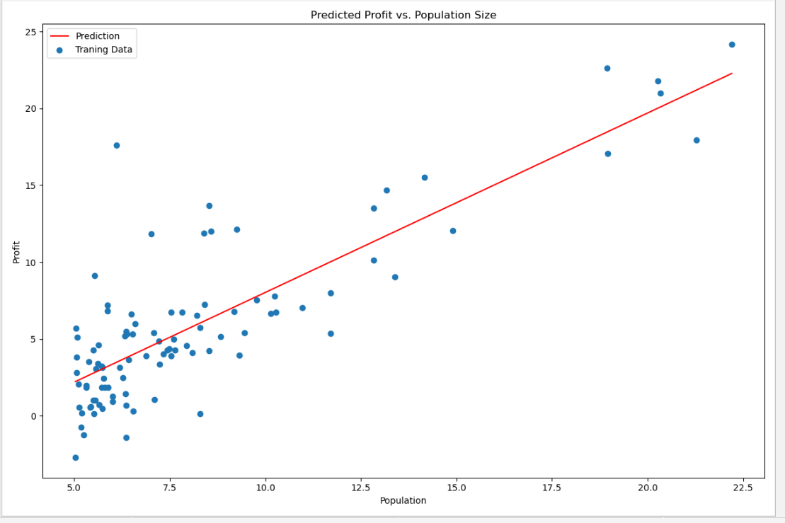
#原始数据以及拟合的直线
# 横坐标轴的取值区间 和 分割点数
x = np.linspace(data.Population.min(), data.Population.max(), 100)
f = g[0, 0] + (g[0, 1] * x)
# 画一个子图 子图的大小为 12 * 8
fig, ax = plt.subplots(figsize=(12,8))
# 红色的线 图例为Prediction
ax.plot(x, f, 'r', label='Prediction')
ax.scatter(data.Population, data.Profit, label='Traning Data')
# 显示图例 loc可以取1 2 3 4 分别代表 第1 2 3 4象限
ax.legend(loc=2)
ax.set_xlabel('Population')
ax.set_ylabel('Profit')
ax.set_title('Predicted Profit vs. Population Size')
plt.show()

　具体解释请看：https://www.heywhale.com/mw/project/5da16a37037db3002d441810

结果截图：