Python机器学习之数据探索可视化库yellowbrick-tutorial

背景介绍

从学sklearn时，除了算法的坎要过，还得学习matplotlib可视化，对我的实践应用而言，可视化更重要一些，然而matplotlib的易用性和美观性确实不敢恭维。陆续使用过plotly、seaborn，最终定格在了Bokeh，因为它可以与Flask完美的结合，数据看板的开发难度降低了很多。

前阵子看到这个库可以较为便捷的实现数据探索，今天得空打算学习一下。原本访问的是英文文档，结果发现已经有人在做汉化，虽然看起来也像是谷歌翻译的，本着拿来主义，少费点精力的精神，就半抄半学，还是发现了一些与文档不太一致的地方。

# http://www.scikit-yb.org/zh/latest/tutorial.html

模型选择教程

在本教程中，我们将查看各种 Scikit-Learn 模型的分数，并使用 Yellowbrick 的可视化诊断工具对其进行比较，以便为我们的数据选择最佳模型。

模型选择三元组

关于机器学习的讨论常常集中在模型选择上。无论是逻辑回归、随机森林、贝叶斯方法，还是人工神经网络，机器学习实践者通常都能很快地展示他们的偏好。这主要是因为历史原因。尽管现代的第三方机器学习库使得各类模型的部署显得微不足道，但传统上，即使是其中一种算法的应用和调优也需要多年的研究。因此，与其他模型相比，机器学习实践者往往对特定的(并且更可能是熟悉的)模型有强烈的偏好。

然而，模型选择比简单地选择“正确”或“错误”算法更加微妙。实践中的工作流程包括:

选择和/或设计最小和最具预测性的特性集
从模型家族中选择一组算法，并且
优化算法超参数以优化性能。

模型选择三元组是由Kumar 等人，在 2015 年的 SIGMOD 论文中首次提出。在他们的论文中，谈论到下一代为预测建模而构建的数据库系统的开发。作者很中肯地表示，由于机器学习在实践中具有高度实验性，因此迫切需要这样的系统。“模型选择，”他们解释道，“是迭代的和探索性的，因为(模型选择三元组)的空间通常是无限的，而且通常不可能让分析师事先知道哪个(组合)将产生令人满意的准确性和/或洞察力。”

最近，许多工作流程已经通过网格搜索方法、标准化 API 和基于 GUI 的应用程序实现了自动化。然而，在实践中，人类的直觉和指导可以比穷举搜索更有效地专注于模型质量。通过可视化模型选择过程，数据科学家可以转向最终的、可解释的模型，并避免陷阱。

Yellowbrick 库是一个针对机器学习的可视化诊断平台，它允许数据科学家控制模型选择过程。Yellowbrick 用一个新的核心对象扩展了Scikit-Learn 的 API: Visualizer。Visualizers 允许可视化模型作为Scikit-Learn管道过程的一部分进行匹配和转换，从而在高维数据的转换过程中提供可视化诊断。

关于数据

本教程使用来自 UCI Machine Learning Repository 的修改过的蘑菇数据集版本。我们的目标是基于蘑菇的特定，去预测蘑菇是有毒的还是可食用的。

这些数据包括与伞菌目(Agaricus)和环柄菇属(Lepiota)科中23种烤蘑菇对应的假设样本描述。每一种都被确定为绝对可食用，绝对有毒，或未知的可食用性和不推荐（后一类与有毒物种相结合）。

我们的文件“agaricus-lepiota.txt”，包含3个名义上有价值的属性信息和8124个蘑菇实例的目标值(4208个可食用，3916个有毒)。

让我们用Pandas加载数据。

import os
import pandas as pd
mushrooms = 'data/shrooms.csv'  # 数据集
dataset   = pd.read_csv(mushrooms)
# dataset.columns = names
dataset.head()

	id	class	cap-shape	cap-surface	cap-color	bruises	odor	gill-attachment	gill-spacing	gill-size	...	stalk-color-above-ring	stalk-color-below-ring	veil-type	veil-color	ring-number	ring-type	spore-print-color	population	habitat	Unnamed: 24
0	1	p	x	s	n	t	p	f	c	n	...	w	w	p	w	o	p	k	s	u	NaN
1	2	e	x	s	y	t	a	f	c	b	...	w	w	p	w	o	p	n	n	g	NaN
2	3	e	b	s	w	t	l	f	c	b	...	w	w	p	w	o	p	n	n	m	NaN
3	4	p	x	y	w	t	p	f	c	n	...	w	w	p	w	o	p	k	s	u	NaN
4	5	e	x	s	g	f	n	f	w	b	...	w	w	p	w	o	e	n	a	g	NaN

5 rows × 25 columns

features = ['cap-shape', 'cap-surface', 'cap-color']
target   = ['class']
X = dataset[features]
y = dataset[target]

dataset.shape # 较官方文档少了俩蘑菇

(8122, 25)

dataset.groupby('class').count() # 各少了1个蘑菇

	id	cap-shape	cap-surface	cap-color	bruises	odor	gill-attachment	gill-spacing	gill-size	gill-color	...	stalk-color-above-ring	stalk-color-below-ring	veil-type	veil-color	ring-number	ring-type	spore-print-color	population	habitat	Unnamed: 24
class
e	4207	4207	4207	4207	4207	4207	4207	4207	4207	4207	...	4207	4207	4207	4207	4207	4207	4207	4207	4207	0
p	3915	3915	3915	3915	3915	3915	3915	3915	3915	3915	...	3915	3915	3915	3915	3915	3915	3915	3915	3915	0

2 rows × 24 columns

特征提取

我们的数据，包括目标参数，都是分类型数据。为了使用机器学习，我们需要将这些值转化为数值型数据。为了从数据集中提取这一点，我们必须使用Scikit-Learn的转换器（transformers）将输入数据集转换为适合模型的数据集。幸运的是，Sckit-Learn提供了一个转换器，用于将分类标签转换为整数: sklearn.preprocessing.LabelEncoder。不幸的是，它一次只能转换一个向量，所以我们必须对它进行调整，以便将它应用于多个列。
有疑问，这个蘑菇分类就是一个向量？

from sklearn.base import BaseEstimator, TransformerMixin
from sklearn.preprocessing import LabelEncoder, OneHotEncoder
class EncodeCategorical(BaseEstimator, TransformerMixin):
    """
    Encodes a specified list of columns or all columns if None.
    """

    def __init__(self, columns=None):
        self.columns  = [col for col in columns]
        self.encoders = None

    def fit(self, data, target=None):
        """
        Expects a data frame with named columns to encode.
        """
        # Encode all columns if columns is None
        if self.columns is None:
            self.columns = data.columns

        # Fit a label encoder for each column in the data frame
        self.encoders = {
            column: LabelEncoder().fit(data[column])
            for column in self.columns
        }
        return self

    def transform(self, data):
        """
        Uses the encoders to transform a data frame.
        """
        output = data.copy()
        for column, encoder in self.encoders.items():
            output[column] = encoder.transform(data[column])

        return output

建模与评估

评估分类器的常用指标

精确度(Precision) 是正确的阳性结果的数量除以所有阳性结果的数量(例如，我们预测的可食用蘑菇实际上有多少?)

召回率(Recall) 是正确的阳性结果的数量除以应该返回的阳性结果的数量(例如，我们准确预测了多少有毒蘑菇是有毒的?)

F1分数(F1 score) 是测试准确度的一种衡量标准。它同时考虑测试的精确度和召回率来计算分数。F1得分可以解释为精度和召回率的加权平均值，其中F1得分在1处达到最佳值，在0处达到最差值。
precision = true positives / (true positives + false positives)

recall = true positives / (false negatives + true positives)

F1 score = 2 * ((precision * recall) / (precision + recall))
现在我们准备好作出一些预测了！

让我们构建一种评估多个估算器(multiple estimators)的方法 —— 首先使用传统的数值分数（我们稍后将与Yellowbrick库中的一些可视化诊断进行比较）。

from sklearn.metrics import f1_score
from sklearn.pipeline import Pipeline
def model_selection(X, y, estimator):
    """
    Test various estimators.
    """
    y = LabelEncoder().fit_transform(y.values.ravel())
    model = Pipeline([
         ('label_encoding', EncodeCategorical(X.keys())),
         ('one_hot_encoder', OneHotEncoder(categories='auto')),  # 此处增加自动分类，否则有warning
         ('estimator', estimator)
    ])

    # Instantiate the classification model and visualizer
    model.fit(X, y)

    expected  = y
    predicted = model.predict(X)

    # Compute and return the F1 score (the harmonic mean of precision and recall)
    return (f1_score(expected, predicted))

from sklearn.svm import LinearSVC, NuSVC, SVC
from sklearn.neighbors import KNeighborsClassifier
from sklearn.linear_model import LogisticRegressionCV, LogisticRegression, SGDClassifier
from sklearn.ensemble import BaggingClassifier, ExtraTreesClassifier, RandomForestClassifier

model_selection(X, y, LinearSVC())

0.6582119537920643

import warnings
warnings.filterwarnings("ignore", category=FutureWarning, module="sklearn")  # 忽略警告

model_selection(X, y, NuSVC())

0.6878837238441299

model_selection(X, y, SVC())

0.6625145971195017

model_selection(X, y, SGDClassifier())

0.5738408700629649

model_selection(X, y, KNeighborsClassifier())

0.6856846473029046

model_selection(X, y, LogisticRegressionCV())

0.6582119537920643

model_selection(X, y, LogisticRegression())

0.6578749058025622

model_selection(X, y, BaggingClassifier())

0.6873901878632248

model_selection(X, y, ExtraTreesClassifier())

0.6872294372294372

model_selection(X, y, RandomForestClassifier())

0.6992081007399714

初步模型评估

根据上面F1分数的结果，哪个模型表现最好？

可视化模型评估

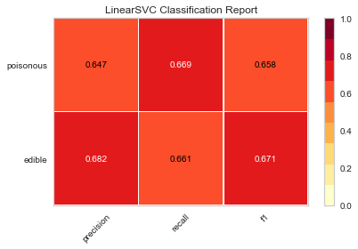
现在，让我们重构模型评估函数，使用Yellowbrick的ClassificationReport类，这是一个模型可视化工具，可以显示精确度、召回率和F1分数。这个可视化的模型分析工具集成了数值分数以及彩色编码的热力图，以支持简单的解释和检测，特别是对于我们用例而言非常相关(性命攸关!)的第一类错误(Type I error)和第二类错误(Type II error)的细微差别。

第一类错误 (或 "假阳性(false positive)" ) 是检测一种不存在的效应(例如，当蘑菇实际上是可以食用的时候，它是有毒的)。

第二类错误 (或 “假阴性”"false negative" ) 是未能检测到存在的效应(例如，当蘑菇实际上有毒时，却认为它是可以食用的)。

from sklearn.pipeline import Pipeline
from yellowbrick.classifier import ClassificationReport


def visual_model_selection(X, y, estimator):
    """
    Test various estimators.
    """
    y = LabelEncoder().fit_transform(y.values.ravel())
    model = Pipeline([
         ('label_encoding', EncodeCategorical(X.keys())),
         ('one_hot_encoder', OneHotEncoder()),
         ('estimator', estimator)
    ])

    # Instantiate the classification model and visualizer
    visualizer = ClassificationReport(model, classes=['edible', 'poisonous'])
    visualizer.fit(X, y)
    visualizer.score(X, y)
    visualizer.poof()

visual_model_selection(X, y, LinearSVC())

file

# 其他分类器可视化略
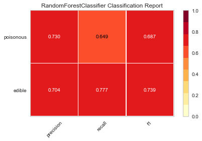
visual_model_selection(X, y, RandomForestClassifier())

file

检验

现在,哪种模型看起来最好?为什么?
哪一个模型最有可能救你的命?
可视化模型评估与数值模型评价，体验起来有何不同?

准确率Precision召回率Recall以及综合评价指标F1-Measure
http://www.makaidong.com/博客园热文/437.shtml
f1-score综合考虑的准确率和召回率。
可视化就是直观嘛，逃~

作者简介

知乎yeayee，Py龄5年，善Flask+MongoDB+SKlearn+Bokeh

posted on 2019-08-20 16:49 yeayee 阅读(884) 评论(0) 编辑收藏举报

刷新页面返回顶部

yeayee