实验一 感知器及其应用

这个作业属于哪个课程	https://edu.cnblogs.com/campus/ahgc/machinelearning
这个作业要求在哪里	https://edu.cnblogs.com/campus/ahgc/machinelearning/homework/11950
这个作业的目标	<理解和实现感知器算法>
学号	<3180701330>

实验一 感知器及其应用

【实验目的】

1. 理解感知器算法原理，能实现感知器算法；

2. 掌握机器学习算法的度量指标；

3. 掌握最小二乘法进行参数估计基本原理；

4. 针对特定应用场景及数据，能构建感知器模型并进行预测。

【实验内容】

1. 安装Pycharm，注册学生版。

2. 安装常见的机器学习库，如Scipy、Numpy、Pandas、Matplotlib，sklearn等。

3. 编程实现感知器算法。

4. 熟悉iris数据集，并能使用感知器算法对该数据集构建模型并应用。

【实验过程及步骤】

代码如下：

import numpy as np
from sklearn.datasets import load_iris #载入Fisher的鸢尾花数据
import matplotlib.pyplot as plt  
#Matplotlib是Python的一个绘图库，是Python中最常用的可视化工具之一，可以非常方便地创建2D图表和一些基本的3D图表pyplot模块的plot函数可以接收输入参数和输出参数，还有线条粗细等参数
%matplotlib inline

iris = load_iris()
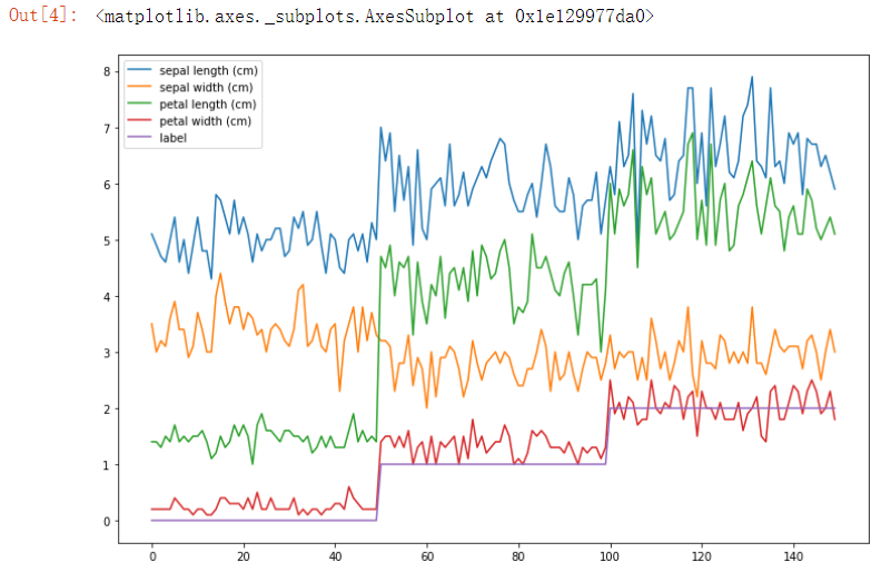
df = pd.DataFrame(iris.data, columns=iris.feature_names) #是一个表格 
df['label'] = iris.target # 表头字段就是key
df.plot(figsize = (12, 8)) # 利用dataframe做简单的可视化分析

df.label.value_counts()

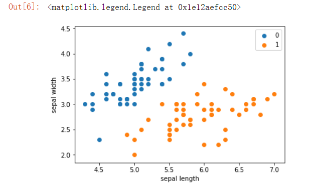
plt.scatter(df[50:100]['sepal length'], df[50:100]['sepal width'], label='1')
plt.xlabel('sepal length')
plt.ylabel('sepal width')
plt.legend()

data = np.array(df.iloc[:100, [0, 1, -1]]) # 取前100条数据，为了方便展示，取2个特征

X, y = data[:,:-1], data[:,-1]  # 数据类型转换，为了后面的数学计算

y = np.array([1 if i == 1 else -1 for i in y])

# 此处为一元一次线性方程
class Model:
    def __init__(self):
        self.w = np.ones(len(data[0])-1, dtype=np.float32)
        self.b = 0 #初始w/b的值
        self.l_rate = 0.1
        # self.data = data
    def sign(self, x, w, b):
        y = np.dot(x, w) + b #求w，b的值
        #Numpy中dot()函数主要功能有两个：向量点积和矩阵乘法。
        #格式：x.dot(y) 等价于 np.dot(x,y) ———x是m*n 矩阵 ，y是n*m矩阵，则x.dot(y) 得到m*m矩阵
        return y
    
    # 随机梯度下降法
    #随机梯度下降法（SGD），随机抽取一个误分类点使其梯度下降。根据损失函数的梯度，对w，b进行更新
    def fit(self, X_train, y_train): #将参数拟合 X_train数据集矩阵 y_train特征向量
        is_wrong = False
        #误分类点的意思就是开始的时候，超平面并没有正确划分，做了错误分类的数据。
        while not is_wrong:
            wrong_count = 0 #误分为0，就不用循环，得到w，b
            for d in range(len(X_train)):
                X = X_train[d]
                y = y_train[d]
                if y * self.sign(X, self.w, self.b) <= 0: 
                    # 如果某个样本出现分类错误，即位于分离超平面的错误侧，则调整参数，使分离超平面开始移动，直至误分类点被正确分类。
                    self.w = self.w + self.l_rate*np.dot(y, X) #调整w和b
                    self.b = self.b + self.l_rate*y
                    wrong_count += 1
            if wrong_count == 0:
                is_wrong = True
        return 'Perceptron Model!'
#线性可分可用随机梯度下降法
    def score(self):
        pass

perceptron = Model()
perceptron.fit(X, y)

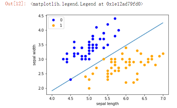
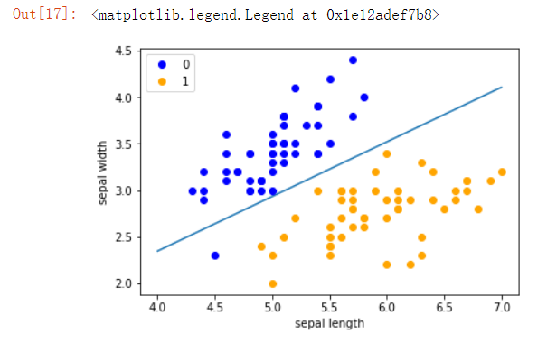
y_ = -(perceptron.w[0]*x_points + perceptron.b)/perceptron.w[1]
plt.plot(x_points, y_)
plt.plot(data[:50, 0], data[:50, 1], 'bo', color='blue', label='0')
plt.plot(data[50:100, 0], data[50:100, 1], 'bo', color='orange', label='1')
plt.xlabel('sepal length')
plt.ylabel('sepal width')
plt.legend()

from sklearn.linear_model import Perceptron

clf = Perceptron(fit_intercept=False, max_iter=1000, shuffle=False)
#得到训练结果，权重矩阵
clf.fit(X,y)

print(clf.coef_)

print(clf.intercept_)

y_ = -(clf.coef_[0][0]*x_ponits + clf.intercept_)/clf.coef_[0][1]
plt.plot(x_ponits, y_)
plt.plot(data[:50, 0], data[:50, 1], 'bo', color='blue', label='0')
plt.plot(data[50:100, 0], data[50:100, 1], 'bo', color='orange', label='1')
plt.xlabel('sepal length')
plt.ylabel('sepal width')
plt.legend()

【实验小结】

当预测值等于我们期待的结果时： 什么也不用做
但当其小于的时候，说明我们增加的权值小了，应补上一个正数数