
线性代数 | 要义 / 本质 (上篇) - 指南
注:本文为 “线性代数 | 要义 / 本质” 相关合辑。
英文引文,机翻未校。
中文引文,略排未全校。
如有内容异常,请看原文。
Essence of linear algebra
线性代数要义
February 2020
Notes on the excellent YouTube series by 3Blue1Brown. This series taught me more about linear algebra than any class in college.
本文是 YouTube 上 3Blue1Brown 频道优质系列视频的学习笔记。该系列视频教给我的线性代数知识,比我在大学任何一门课上学到的都多。
(I wrote these to help reinforce the concepts from the series. It may be useful as a supplement, but it’s no substitute for the animations themselves.)
(我撰写这些笔记是为了巩固该系列视频中的概念。笔记或许能作为有益补充,但无法替代视频本身的动画演示。)
What are vectors?
向量是什么?
A vector can describe anything where there is a sensible notion of adding vectors and multiplying vectors by numbers.
只要某个事物存在“向量相加”和“向量与数相乘”的合理定义,就可以用向量来描述它。
Vectors are scaled by scalars, which are numbers, or constants.
向量可利用标量(即数字或常数)进行缩放。
In the physics world, vectors are often thought of as arrows in space, with direction and magnitude.
在物理学领域,向量通常被视为空间中的箭头,具有方向和大小两个属性。
In the computer science world, vectors are often lists of numbers (scalars).
在计算机科学领域,向量通常是数字(标量)的列表。
Both of these perspectives can provide a useful framework for understanding vectors. This series will focus on deepening one’s intuition via geometric interpretations.
这两种视角都能为理解向量给出有用的框架。本系列视频将着重通过几何解释来深化对向量的直观认知。
Linear combinations, span, and basis vectors
线性组合、张成空间与基向量
The coordinates of a vector can be thought of as scalars of some unit vectors. Those unit vectors are the basis vectors for the given vector space.
向量的坐标可视为某些单位向量的标量倍数,这些单位向量就是给定向量空间的基向量。
- Any time you describe vectors numerically, it depends on an implicit choice of basis vectors.
任何时候,当你用数值描述向量时,都依赖于对基向量的一个隐含选择。
A linear combination of vectors is the result of a scalar multiplication and element-wise vector addition. For vectorsv
⃗
\vec{v}v and w
⃗
\vec{w}w:
向量的线性组合是标量乘法与向量按元素相加的结果。对于向量v
⃗
\vec{v}v 和 w
⃗
\vec{w}w,有:
a
v
⃗
+
b
w
⃗
=
[
a
v
1
+
b
w
1
a
v
2
+
b
w
2
⋯
a
v
n
+
b
w
n
]
a \vec{v} + b \vec{w} = \begin{bmatrix} a v_1 + b w_1 \\ a v_2 + b w_2 \\ \cdots \\ a v_n + b w_n \end{bmatrix}av+bw=av1+bw1av2+bw2⋯avn+bwn
where a
aa and b
bbvary over the real numbersR
\mathbb{R}R.
其中,a
aa 和 b
bb是取值范围为实数集R
\mathbb{R}R 的变量。
The span of a set of vectors is the set formed by all of their linear combinations. Geometrically, it can be easier to think about a vector as an arrow, and the span of that vector as the line drawn by that arrow in either direction, i.e. scaled up and down by any scalar.
由该箭头向两个方向延伸所形成的直线(即通过任意标量对向量进行缩放得到的所有向量)。就是一组向量的张成空间,是由这组向量的所有线性组合构成的集合。从几何角度理解更简便:将单个向量视为箭头,其张成空间就
This also extends to higher dimensions, e.g. a plane or hyperplane.
这一概念也可推广到更高维度,例如平面或超平面。
A vector is linearly dependent to a set of vectors if it is a linear combination of those vectors. In other words, it is linearly dependent if its removal from the set does not affect the span of that set (it lies somewhere on the span).
某组向量的线性组合,则该向量与这组向量线性相关。换句话说,若从这组向量中移除该向量后,集合的张成空间不变(即该向量落在原集合的张成空间内),则称其与这组向量线性相关。就是若一个向量
A basis of a vector space is a set of linearly independent vectors that spans the full space.
向量空间的基,是一组能够张成整个空间的线性无关向量。
Linear transformations and matrices
线性变换与矩阵
A linear transformation is a transformation function that accepts and returns a vector. To respect linearity, a transformation must:
一种接收向量并返回向量的变换函数。要满足“线性”,变换必须满足以下两个条件:就是线性变换
- preserve all lines
保持所有直线不变(不弯曲) - preserve the origin
保持原点位置不变
A transformation from one coordinate system to another can be described with ann
nn-dimensional transformation matrix, where the matrix is a set of vectors lined up in columns. Conversely, all matrices can also be thought of as transformations.
从一个坐标系到另一个坐标系的变换,可以用一个n
nn维变换矩阵来描述——该矩阵由一组向量按列排列构成。反过来,所有矩阵也都可视为某种线性变换的表示。
For example, consider a vectorv
⃗
=
[
x
,
y
]
\vec{v} = [x, y]v=[x,y], defined in the standard 2D coordinate-plane. Think ofv
⃗
\vec{v}vas a linear combination of the “implicit” standard basis vectorsi
^
=
[
1
,
0
]
\hat{i} = [1, 0]i^=[1,0] and j
^
=
[
0
,
1
]
\hat{j} = [0, 1]j^=[0,1], i.e.v
⃗
=
x
i
^
+
y
j
^
\vec{v} = x \hat{i} + y \hat{j}v=xi^+yj^.
例如,考虑在标准二维坐标平面中定义的向量v
⃗
=
[
x
,
y
]
\vec{v} = [x, y]v=[x,y]。可将 v
⃗
\vec{v}v视为“隐含的”标准基向量i
^
=
[
1
,
0
]
\hat{i} = [1, 0]i^=[1,0] 和 j
^
=
[
0
,
1
]
\hat{j} = [0, 1]j^=[0,1]的线性组合,即v
⃗
=
x
i
^
+
y
j
^
\vec{v} = x \hat{i} + y \hat{j}v=xi^+yj^。
Now, apply a linear transformation to the entire coordinate system, movingi
^
\hat{i}i^ and j
^
\hat{j}j^. This transformation can be described by a(
2
,
2
)
(2, 2)(2,2)matrixA
AA, where the first column is the resulting coordinates of the basis vectori
⃗
=
[
a
,
b
]
\vec{i} = [a, b]i=[a,b], and the second column is the resulting coordinates of the basis vectorj
⃗
=
[
c
,
d
]
\vec{j} = [c, d]j=[c,d].
现在,对整个坐标系施加一个线性变换,使基向量i
^
\hat{i}i^ 和 j
^
\hat{j}j^移动到新位置。该变换可用一个(
2
,
2
)
(2, 2)(2,2) 矩阵 A
AA描述:矩阵的第一列是基向量i
⃗
\vec{i}i变换后的坐标[
a
,
b
]
[a, b][a,b]基向量就是,第二列j
⃗
\vec{j}j变换后的坐标[
c
,
d
]
[c, d][c,d]。
If you apply that transformation to vectorv
⃗
\vec{v}v, by performing the multiplicationA
v
⃗
A\vec{v}Av, the result is the same linear combinationx
i
⃗
+
y
j
⃗
x \vec{i} + y \vec{j}xi+yj!
若通过矩阵乘法A
v
⃗
A\vec{v}Av 对向量 v
⃗
\vec{v}v施加该变换,得到的结果与线性组合x
i
⃗
+
y
j
⃗
x \vec{i} + y \vec{j}xi+yj 完全相同!
[
a
c
b
d
]
[
x
y
]
=
x
[
a
b
]
+
y
[
c
d
]
⏟
where all the intuition is
=
[
a
x
+
c
y
b
x
+
d
y
]
\begin{bmatrix} a & c \\ b & d \end{bmatrix} \begin{bmatrix} x \\ y \end{bmatrix} = \underbrace{ x \begin{bmatrix} a \\ b \end{bmatrix} + y \begin{bmatrix} c \\ d \end{bmatrix} }_{\text{where all the intuition is}} = \begin{bmatrix} ax + cy \\ bx + dy \end{bmatrix}[abcd][xy]=where all the intuition isx[ab]+y[cd]=[ax+cybx+dy]
Matrix multiplication as composition
作为复合操作的矩阵乘法
Matrix multiplication can be interpreted geometrically as the composition of linear transformations.
从几何角度看,矩阵乘法可解释为线性变换的复合(即先后施加多个线性变换)。
For example, to apply a rotation and a shear to a 2D vector, we could apply each one successively. But since both of these operations are linear transformations, we know that each basis vectori
^
\hat{i}i^ and j
^
\hat{j}j^will land at some new coordinatesi
⃗
\vec{i}i and j
⃗
\vec{j}jin the 2D plane. This means we can describe both operations with a single, composed(
2
,
2
)
(2, 2)(2,2)transformation matrix.
线性变换,基向量就是例如,要对一个二维向量先后施加旋转变换和剪切变换,可依次执行这两个操控。但由于这两个操作都i
^
\hat{i}i^ 和 j
^
\hat{j}j^最终会落在二维平面中的新坐标i
⃗
\vec{i}i 和 j
⃗
\vec{j}j处。这意味着我们可用一个单一的复合(
2
,
2
)
(2, 2)(2,2)变换矩阵来描述这两个操作的整体效果。
Note that matrix multiplication moves right-to-left, as if each operation were a function being applied to the result of an inner function, e.g.f
(
g
(
h
(
x
)
)
)
f(g(h(x)))f(g(h(x))). In other words, it is associative, but not commutative.
需注意,矩阵乘法的执行顺序是从右到左,就像每个变换都是作用于“内层函数结果”的函数(例如f
(
g
(
h
(
x
)
)
)
f(g(h(x)))f(g(h(x)))的执行顺序是先h
hh、再 g
gg、最后 f
ff)。换句话说,矩阵乘法满足结合律,但不满足交换律。
The determinant
行列式
Given a 2D matrixA
AA, the determinant represents the factor by which area is scaled by the transformation specified byA
AA. Negative determinants describe inverted orientations, though the absolute value is still the scale factor.
对于二维矩阵A
AA,其行列式表示该矩阵所对应的线性变换对“面积”的缩放比例。负的行列式表示变换后空间的定向发生翻转,但行列式的绝对值仍为面积的缩放比例。
To figure out if the determinant will be negative, recall that the identity matrix has a determinant of1
11. So if the relative positioning ofi
^
\hat{i}i^is clockwise fromj
^
\hat{j}j^, the orientation is positive.
否为负,可回顾:单位矩阵的行列式为就是要判断行列式1
11。若变换后基向量i
^
\hat{i}i^ 相对于 j
^
\hat{j}j^的位置关系为顺时针,则空间定向为正(行列式为正);反之则定向为负(行列式为负)。
Similarly, in 3D, the determinant of a matrix represents the transformation’s scale factor for volume, and the sign of the orientation is indicated by the right-hand rule (pointer finger isi
^
\hat{i}i^, middle finger isj
^
\hat{j}j^, thumb isk
^
\hat{k}k^).
类似地,在三维空间中,矩阵的行列式表示变换对“体积”的缩放比例;空间定向的正负则借助右手定则判断(食指指向i
^
\hat{i}i^方向,中指指向j
^
\hat{j}j^方向,拇指指向k
^
\hat{k}k^ 方向)。
A matrix with a determinant of0
00indicates that the transformation projects the vector into a lower-dimensional space.
行列式为 0
00的矩阵,表示其对应的线性变换会将向量投影到更低维度的空间中(例如,二维空间投影到一维直线,三维空间投影到二维平面)。
Due to the compositionality of matrix multiplication, if you multiply two matrices together, the determinant of the resulting matrix is equal to the product of the determinants of the original two matrices, i.e.d
e
t
(
A
1
A
2
)
=
d
e
t
(
A
1
)
d
e
t
(
A
2
)
det(A_1 A_2) = det(A_1) det(A_2)det(A1A2)=det(A1)det(A2).
由于矩阵乘法具有复合性,若将两个矩阵相乘,所得矩阵的行列式等于原来两个矩阵行列式的乘积,即d
e
t
(
A
1
A
2
)
=
d
e
t
(
A
1
)
d
e
t
(
A
2
)
det(A_1 A_2) = det(A_1) det(A_2)det(A1A2)=det(A1)det(A2)。
Inverse matrices, column space and null space
逆矩阵、列空间与零空间
Matrices can be used to solve linear systems of equations. These must be expressable in the form of linear combinations of basis vectors.
矩阵可用于求解线性方程组,而线性方程组必须能表示为基向量的线性组合形式。
The inverse matrixA
−
1
A^{-1}A−1 of A
AAis the unique matrix with the property thatA
−
1
A
=
I
A^{-1}A = IA−1A=I, whereI
IIis the identity matrix (1
11s along the diagonal,0
00s everywhere else). That is,A
−
1
A^{-1}A−1is the transformation that will “undo” the transformationA
AA.
矩阵 A
AA 的逆矩阵 A
−
1
A^{-1}A−1 是满足 A
−
1
A
=
I
A^{-1}A = IA−1A=I的唯一矩阵,其中I
II是单位矩阵(对角线元素为1
11,其余元素为0
00)。也就是说,A
−
1
A^{-1}A−1对应的线性变换能“撤销”矩阵A
AA对应的线性变换。
If a matrixA
AAhas a determinant of0
00, then its inverse does not exist. There is no way to invert a transformation from a higher dimension to a lower dimension.
若矩阵 A
AA 的行列式为 0
00无法“撤销”的。就是,则其逆矩阵不存在。这是因为,将高维空间投影到低维空间的变换
- If a line is projected to a point, how would you know which line to draw to “uncompress” it?
例如,若一条直线被投影成一个点,你无法确定应该画出哪一条直线才能“还原”它。
The rank of a matrix is the number of dimensions in the output of its transformation. For example, if a linear transformation results in a line, its matrix has a rank of1
11. If the output is a plane, it has a rank of2
22.
一条直线(一维),则矩阵的秩为就是矩阵的秩,是其对应的线性变换输出空间的维度。例如,若线性变换的输出1
11;若输出是一个平面(二维),则矩阵的秩为2
22。
A full rank matrix preserves the number of dimensions of its input.
满秩矩阵能保持输入空间的维度(即变换后空间维度与原空间维度相同)。
The column space of a matrixA
AAis the set of all possible outputsA
v
⃗
A \vec{v}Av, v
⃗
∈
R
\vec{v} \in \mathbb{R}v∈R. That is, the column space ofA
AAis the span of the columns ofA
AA.
矩阵 A
AA的列空间,是所有可能的输出A
v
⃗
A \vec{v}Av(其中 v
⃗
∈
R
\vec{v} \in \mathbb{R}v∈R说,矩阵就是)构成的集合。也就A
AA的列空间等于其各列向量所张成的空间。
Therefore, the rank of a matrix can be thought of as the dimensionality of its column space.
因此,矩阵的秩也可理解为其列空间的维度。
Any matrix which is not full rank has a null space, or kernel. The null space of a matrix is the vector space which is transformed to the origin.
所有非满秩矩阵都存在零空间(也称为核)。矩阵的零空间,是所有经过变换后映射到原点的向量构成的空间。
In any full rank transformation, only the zero-vector outputs the origin (any linear transformation must preserve the origin).
在满秩变换中,只有零向量会被映射到原点(所有线性变换都必须保持原点不变)。In any non-full rank transformation, there is a set of vectors that will be transformed to the origin. For example, if a 2D matrix “compresses” a plane to a line, there exists some line in the original plane which was entirely mapped to the origin.
在非满秩变换中,存在一组向量会被映射到原点。例如,若一个二维矩阵将平面“压缩”成一条直线,则原平面中存在某条直线上的所有向量,都会被映射到原点。
In the context of linear system of equations,A
x
⃗
=
v
⃗
A\vec{x} = \vec{v}Ax=v, if v
⃗
=
0
\vec{v} = 0v=0, the null space ofA
AAgives you all possible solutions to the equation.
在线性方程组A
x
⃗
=
v
⃗
A\vec{x} = \vec{v}Ax=v 中,若 v
⃗
=
0
\vec{v} = 0v=0(即齐次线性方程组),则矩阵A
AA的零空间就是该方程组的所有解构成的集合。
Nonsquare matrices as transformations between dimensions
作为维度间变换的非方阵
Nonsquare matrices represent transformations between dimensions. For example, the matrix
非方阵表示不同维度空间之间的线性变换。例如,矩阵
A
=
[
2
0
−
1
1
2
1
]
A = \begin{bmatrix} 2 & 0 \\ -1 & 1 \\ 2 & 1 \end{bmatrix}A=2−12011
represents a transformation from 2D to 3D space.
表示从二维空间到三维空间的线性变换。
The columns still represent the transformed coordinates of the basis vectors—observe that there are two basis vectors, and they each land on coordinates which have three dimensions.
非方阵的列向量仍表示基向量变换后的坐标——需注意,这里有两个基向量(对应输入的二维空间),每个基向量变换后的坐标都有三个维度(对应输出的三维空间)。
This is a full rank matrix, since the resulting vector space is a plane in 3D space.
该矩阵是满秩矩阵,基于其变换后的输出空间是三维空间中的一个平面(维度等于输入空间的维度2
22)。
Dot products and duality
点积与对偶性
The dot product of two vectorsv
⃗
\vec{v}v and w
⃗
\vec{w}wis the result of multiplying the length ofv
⃗
\vec{v}vby the length of the projection ofw
⃗
\vec{w}w onto v
⃗
\vec{v}v.
两个向量 v
⃗
\vec{v}v 和 w
⃗
\vec{w}w的点积,等于v
⃗
\vec{v}v 的长度与 w
⃗
\vec{w}w 在 v
⃗
\vec{v}v上投影长度的乘积。
This computation is symmetric:v
⃗
⋅
w
⃗
=
w
⃗
⋅
v
⃗
\vec{v} \cdot \vec{w} = \vec{w} \cdot \vec{v}v⋅w=w⋅v. Scaling either vector results in a proportional scaling in the projected space of the other vector, i.e.(
2
v
⃗
)
⋅
w
⃗
=
2
(
v
⃗
⋅
w
⃗
)
(2 \vec{v}) \cdot \vec{w} = 2 (\vec{v} \cdot \vec{w})(2v)⋅w=2(v⋅w).
点积的计算具有对称性:v
⃗
⋅
w
⃗
=
w
⃗
⋅
v
⃗
\vec{v} \cdot \vec{w} = \vec{w} \cdot \vec{v}v⋅w=w⋅v。对任意一个向量进行缩放,点积结果会按相同比例缩放,例如(
2
v
⃗
)
⋅
w
⃗
=
2
(
v
⃗
⋅
w
⃗
)
(2 \vec{v}) \cdot \vec{w} = 2 (\vec{v} \cdot \vec{w})(2v)⋅w=2(v⋅w)。
The dot product is often used as a measure of similarity between vectors. If we defineθ
\thetaθto be the angle between two vectorsv
⃗
\vec{v}v and w
⃗
\vec{w}w, then:
点积常被用作衡量向量间相似性的指标。若定义θ
\thetaθ 为向量 v
⃗
\vec{v}v 与 w
⃗
\vec{w}w之间的夹角,则有:
- θ
=
9
0
∘
⇒
v
⃗
⋅
w
⃗
=
0
\theta = 90^\circ \Rightarrow \vec{v} \cdot \vec{w} = 0θ=90∘⇒v⋅w=0
⇒ \Rightarrow⇒ 此时点积为 0 00,说明两向量正交(垂直) - θ
<
9
0
∘
⇒
v
⃗
⋅
w
⃗
>
0
\theta < 90^\circ \Rightarrow \vec{v} \cdot \vec{w} > 0θ<90∘⇒v⋅w>0
⇒ \Rightarrow⇒此时点积为正,说明两向量“相似”(夹角为锐角) - θ
>
9
0
∘
⇒
v
⃗
⋅
w
⃗
<
0
\theta > 90^\circ \Rightarrow \vec{v} \cdot \vec{w} < 0θ>90∘⇒v⋅w<0
⇒ \Rightarrow⇒此时点积为负,说明两向量“反向”(夹角为钝角)
Operationally, the dot product can be computed by element-wise multiplication and then addition, i.e.
从计算角度,点积可通过“按元素相乘后求和”得到,即:
v
⃗
⋅
w
⃗
=
v
1
w
1
+
v
2
w
2
+
⋯
+
v
n
w
n
\vec{v} \cdot \vec{w} = v_1 w_1 + v_2 w_2 + \cdots + v_n w_nv⋅w=v1w1+v2w2+⋯+vnwn
or via the geometric definition:
也可通过几何定义计算:
v
⃗
⋅
w
⃗
=
∥
v
⃗
∥
∥
w
⃗
∥
cos
θ
\vec{v} \cdot \vec{w} = \lVert \vec{v} \rVert \lVert \vec{w} \rVert \cos \thetav⋅w=∥v∥∥w∥cosθ
Duality: a vector of lengthn
nncan be considered a(
1
,
n
)
(1, n)(1,n)matrix. Any vector inherently represents a transformation matrix onto the number line of its span.
对偶性:一个n
nn维向量可视为一个(
1
,
n
)
(1, n)(1,n)矩阵(行矩阵)。本质上,任意向量都对应一个“将空间映射到其张成数轴”的变换矩阵。
This is easiest to understand with a 2D vectoru
⃗
\vec{u}u, which can be written as a(
1
,
2
)
(1, 2)(1,2)matrix[
u
x
,
u
y
]
[u_x, u_y][ux,uy]. The columns of the matrix are where the basis vectorsi
^
,
j
^
\hat{i}, \hat{j}i^,j^land in this transformation.
以二维向量 u
⃗
\vec{u}u为例理解最直观:它可表示为(
1
,
2
)
(1, 2)(1,2) 行矩阵 [
u
x
,
u
y
]
[u_x, u_y][ux,uy],该矩阵的列对应基向量i
^
,
j
^
\hat{i}, \hat{j}i^,j^在这个变换后的位置。
Observe that a dot product with a vectoru
⃗
\vec{u}u:
注意到,向量u
⃗
\vec{u}u与另一向量的点积:
[
u
x
u
y
]
⋅
[
x
y
]
=
u
x
⋅
x
+
u
y
⋅
y
\begin{bmatrix} u_x \\ u_y \end{bmatrix} \cdot \begin{bmatrix} x \\ y \end{bmatrix} = u_x \cdot x + u_y \cdot y[uxuy]⋅[xy]=ux⋅x+uy⋅y
is equivalent to the matrix-vector product, or the length of the vector’s projection ontou
⃗
\vec{u}u, scaled by the length ofu
⃗
\vec{u}u:
等价于行矩阵与列向量的乘法,也等价于“向量在u
⃗
\vec{u}u上的投影长度”乘以“u
⃗
\vec{u}u 的长度”:
[
u
x
u
y
]
[
x
y
]
=
u
x
⋅
x
+
u
y
⋅
y
\begin{bmatrix} u_x & u_y \end{bmatrix} \begin{bmatrix} x \\ y \end{bmatrix} = u_x \cdot x + u_y \cdot y[uxuy][xy]=ux⋅x+uy⋅y
In different applications, it may be informative to think about vectors as the embodiment of a linear transformation.
在不同应用场景中,将向量视为线性变换的具体体现,可能会带来新的理解视角。
Cross products
叉积
The cross product is a binary operation on two 3D vectors,v
⃗
×
w
⃗
\vec{v} \times \vec{w}v×w, producing a vector perpendicular to bothv
⃗
\vec{v}v and w
⃗
\vec{w}w. The output vector has a length equal to the area of the parallelogram enclosed by lining up copies ofv
⃗
\vec{v}v and w
⃗
\vec{w}wtail to tip.
针对两个三维向量的二元运算,记为就是叉积v
⃗
×
w
⃗
\vec{v} \times \vec{w}v×w,运算结果是一个同时垂直于v
⃗
\vec{v}v 和 w
⃗
\vec{w}w的向量。该输出向量的长度等于“将v
⃗
\vec{v}v 和 w
⃗
\vec{w}w首尾相接所构成的平行四边形”的面积。
As with the determinant, order matters, and the sign of the cross product depends on the orientation. We can use the right-hand rule to determine if the orientation is positive or negative.
与行列式类似,叉积的运算顺序会影响结果:叉积的正负由空间定向决定,可依据右手定则判断定向的正负(右手四指从v
⃗
\vec{v}v 绕向 w
⃗
\vec{w}w,拇指方向即为叉积向量的正方向)。
The numeric computation can be formulated as follows: set the standard basis vectors[
i
^
,
j
^
,
k
^
]
[\hat{i}, \hat{j}, \hat{k}][i^,j^,k^]to the first column of a(
3
,
3
)
(3, 3)(3,3)matrix, and setv
⃗
\vec{v}v and w
⃗
\vec{w}wto be the second and third columns. The cross product ofv
⃗
\vec{v}v and w
⃗
\vec{w}wis the determinant of this matrix:
叉积的数值计算可按以下方式推导:构造一个(
3
,
3
)
(3, 3)(3,3)矩阵,第一列为标准基向量[
i
^
,
j
^
,
k
^
]
[\hat{i}, \hat{j}, \hat{k}][i^,j^,k^],第二列为向量v
⃗
\vec{v}v,第三列为向量w
⃗
\vec{w}w,则 v
⃗
\vec{v}v 与 w
⃗
\vec{w}w的叉积等于该矩阵的行列式:
v
⃗
×
w
⃗
=
d
e
t
(
[
i
^
v
1
w
1
j
^
v
2
w
2
k
^
v
3
w
3
]
)
=
i
^
(
v
2
w
3
−
v
3
w
2
)
+
j
^
(
v
3
w
1
−
v
1
w
3
)
+
k
^
(
v
1
w
2
−
v
2
w
1
)
\vec{v} \times \vec{w} = det \left( \begin{bmatrix} \hat{i} & v_1 & w_1 \\ \hat{j} & v_2 & w_2 \\ \hat{k} & v_3 & w_3 \end{bmatrix} \right) = \hat{i}(v_2 w_3 - v_3 w_2) + \hat{j}(v_3 w_1 - v_1 w_3) + \hat{k}(v_1 w_2 - v_2 w_1)v×w=deti^j^k^v1v2v3w1w2w3=i^(v2w3−v3w2)+j^(v3w1−v1w3)+k^(v1w2−v2w1)
Or in simpler terms:
也可简化为如下形式:
[
v
1
v
2
v
3
]
×
[
w
1
w
2
w
3
]
=
[
v
2
w
3
−
v
3
w
2
v
3
w
1
−
v
1
w
3
v
1
w
2
−
v
2
w
1
]
\begin{bmatrix} v_1 \\ v_2 \\ v_3 \end{bmatrix} \times \begin{bmatrix} w_1 \\ w_2 \\ w_3 \end{bmatrix} = \begin{bmatrix} v_2 w_3 - v_3 w_2 \\ v_3 w_1 - v_1 w_3 \\ v_1 w_2 - v_2 w_1 \end{bmatrix}v1v2v3×w1w2w3=v2w3−v3w2v3w1−v1w3v1w2−v2w1
An alternate name for the cross product is the “vector product”, which differentiates it from the dot product or “scalar product”.
叉积的另一个名称是“向量积”,以此与点积(又称“标量积”)区分——叉积结果是向量,点积结果是标量。
The closer two vectors are in orientation, the smaller the cross product between them. The more perpendicular they are, the larger the cross product. This follows from the fact that a skinny parallelogram has a much smaller area than a square.
两个向量的方向越接近,它们的叉积长度越小;方向越垂直,叉积长度越大。这一规律源于几何特性:狭长的平行四边形面积远小于边长相同的正方形面积(当两向量垂直时,平行四边形即为矩形,面积最大)。
Cross products in the light of linear transformations
从线性变换视角看叉积
Reframing the cross product’s formula as a linear transformation can connect the dots to its geometric interpretation.
将叉积公式重新表述为线性变换,能更好地关联其几何意义。
Fix input vectorsv
⃗
\vec{v}v and w
⃗
\vec{w}win 3D space. Place a third variable vectoru
⃗
\vec{u}uanchored at the origin. Consider the parallelepiped thatu
⃗
\vec{u}uforms along withv
⃗
\vec{v}v and w
⃗
\vec{w}w.
固定三维空间中的两个输入向量v
⃗
\vec{v}v 和 w
⃗
\vec{w}w,再引入一个以原点为起点的可变向量u
⃗
\vec{u}u。此时,u
⃗
\vec{u}u、v
⃗
\vec{v}v、w
⃗
\vec{w}w可构成一个平行六面体(由三个相邻边向量张成的立体)。
Definef
(
u
⃗
)
f(\vec{u})f(u)to be a function which returns the volume of this parallelepiped as a function ofu
⃗
\vec{u}u. This function maps 3D space to 1D space. It is also linear, as the volume of the parallelepiped is determined by the formula
定义函数 f
(
u
⃗
)
f(\vec{u})f(u),其输出为“由u
⃗
\vec{u}u、v
⃗
\vec{v}v、w
⃗
\vec{w}w构成的平行六面体”的体积,该函数将三维空间映射到一维空间(体积为标量)。由于平行六面体的体积公式为:
V
=
(
area of the base
)
⋅
(
height
)
V = (\text{area of the base}) \cdot (\text{height})V=(area of the base)⋅(height)
(体积 = 底面积 × 高)
and only the dimension of height varies as a function ofu
⃗
\vec{u}u.
其中,底面积由固定向量v
⃗
\vec{v}v 和 w
⃗
\vec{w}w决定(为定值),只有“高”会随可变向量u
⃗
\vec{u}u的变化而变化,因此f
(
u
⃗
)
f(\vec{u})f(u)是线性函数。
Thus, there exists a(
1
,
3
)
(1, 3)(1,3)matrix that represents this function as a transformation ofu
⃗
\vec{u}u. This matrix has a dual vector, which we can callp
⃗
\vec{p}p. So we can redefine the functionf
(
u
⃗
)
f(\vec{u})f(u), from a matrix-vector product to the dot productp
⃗
⋅
u
⃗
\vec{p} \cdot \vec{u}p⋅u.
根据线性变换的性质,存在一个(
1
,
3
)
(1, 3)(1,3)行矩阵,可表示该函数对u
⃗
\vec{u}u的变换。该矩阵对应一个对偶向量p
⃗
\vec{p}p,因此函数 f
(
u
⃗
)
f(\vec{u})f(u)可从“矩阵-向量乘法”重新定义为“点积p
⃗
⋅
u
⃗
\vec{p} \cdot \vec{u}p⋅u”。
This vectorp
⃗
\vec{p}pis the cross product.p
⃗
\vec{p}pmust have the property that for any vectoru
⃗
\vec{u}u, the dot productp
⃗
⋅
u
⃗
\vec{p} \cdot \vec{u}p⋅uis the volume of the resulting parallelipiped betweenu
⃗
\vec{u}u, v
⃗
\vec{v}v, and w
⃗
\vec{w}w.
这个对偶向量p
⃗
\vec{p}p 就是 v
⃗
\vec{v}v 与 w
⃗
\vec{w}w 的叉积。p
⃗
\vec{p}p具有如下性质:对任意向量u
⃗
\vec{u}u,点积 p
⃗
⋅
u
⃗
\vec{p} \cdot \vec{u}p⋅u 的结果等于 u
⃗
\vec{u}u、v
⃗
\vec{v}v、w
⃗
\vec{w}w所构成的平行六面体的体积。
The geometric interpretation: the dot productp
⃗
⋅
u
⃗
\vec{p} \cdot \vec{u}p⋅uis the projection ofu
⃗
\vec{u}u onto p
⃗
\vec{p}p, multiplied by the length ofp
⃗
\vec{p}p. If the length ofp
⃗
\vec{p}pis set to the area of the base (the parallelogram formed byv
⃗
\vec{v}v and w
⃗
\vec{w}w) and p
⃗
\vec{p}pis oriented to be perpendicular tov
⃗
\vec{v}v and w
⃗
\vec{w}wsuch that the right-hand-rule is satisfied, we can see that the dot product formula matches the previous formula for volume:
几何意义解读:点积p
⃗
⋅
u
⃗
\vec{p} \cdot \vec{u}p⋅u 等于“u
⃗
\vec{u}u 在 p
⃗
\vec{p}p上的投影长度”乘以“p
⃗
\vec{p}p的长度”。若将p
⃗
\vec{p}p的长度设为“v
⃗
\vec{v}v 和 w
⃗
\vec{w}w构成的平行四边形底面积”,且让p
⃗
\vec{p}p 垂直于 v
⃗
\vec{v}v 和 w
⃗
\vec{w}w并满足右手定则,则点积公式与平行六面体体积公式完全一致:
(
area of the base
)
⋅
(
height
)
=
(
∥
p
⃗
∥
)
⋅
(
∥
u
⃗
∥
cos
θ
)
(\text{area of the base}) \cdot (\text{height}) = (\lVert \vec{p} \rVert) \cdot (\lVert \vec{u} \rVert \cos \theta)(area of the base)⋅(height)=(∥p∥)⋅(∥u∥cosθ)
(底面积 × 高 =p
⃗
\vec{p}p 的长度 × u
⃗
\vec{u}u 在 p
⃗
\vec{p}p上的投影长度)
Beautiful!
这一对应关系很精妙!
Cramer’s rule
克拉默法则
Cramer’s rule is a method to solve for just one of the variables of a linear system of equationsA
x
⃗
=
v
⃗
A\vec{x} = \vec{v}Ax=v, which doesn’t require the inverse matrixA
−
1
A^{-1}A−1.
克拉默法则是求解线性方程组A
x
⃗
=
v
⃗
A\vec{x} = \vec{v}Ax=v中某一个变量的方法,无需计算逆矩阵A
−
1
A^{-1}A−1。
- Note: Cramer’s rule is useful for deepening one’s intuition for linear systems, but practically will always be slower than Gaussian elimination.
注:克拉默法则有助于深化对线性方程组的直观理解,但在实际计算中,其效率远低于高斯消元法。
A linear transformation that preserves the output of dot products is orthonormal:
若一个线性变换能保持点积结果不变,则该变换是“正交归一”的,满足:
T
(
v
⃗
)
⋅
T
(
w
⃗
)
=
v
⃗
⋅
w
⃗
,
∀
v
⃗
,
w
⃗
T(\vec{v}) \cdot T(\vec{w}) = \vec{v} \cdot \vec{w}, \; \forall \vec{v}, \vec{w}T(v)⋅T(w)=v⋅w,∀v,w
(对任意向量v
⃗
\vec{v}v、w
⃗
\vec{w}w,变换后向量的点积等于原向量的点积)
Geometrically, this involves intuition about how an arbitrary space (area, volume, etc.) is scaled via the determinant of the matrixA
AA, and comparing the untransformed area (parallelogram, parallelopiped, etc.) to the transformed area.
从几何角度,正交归一变换的核心直观认知是:矩阵A
AA的行列式决定了空间(面积、体积等)的缩放比例,且变换前后“平行四边形(或平行六面体)的面积(或体积)比例”可通过行列式关联。
Change of basis
基变换
A change of basis is a transformation from one coordinate system to another.
基变换是指从一个坐标系转换到另一个坐标系的过程。
Consider the matrixA
AAdefined in our standard coordinate system, with columns equal to a 2nd coordinate system’s basis vectors. For example, with our basis vectorsi
^
=
[
1
,
0
]
\hat{i} = [1, 0]i^=[1,0] and j
^
=
[
0
,
1
]
\hat{j} = [0, 1]j^=[0,1], and another system’s basis vectorsi
^
2
=
[
2
,
1
]
\hat{i}_2 = [2, 1]i^2=[2,1] and j
^
2
=
[
−
1
,
1
]
\hat{j}_2 = [-1, 1]j^2=[−1,1], then
假设在标准坐标系中定义矩阵A
AA,其列向量为“第二个坐标系的基向量”。例如,标准坐标系的基向量为i
^
=
[
1
,
0
]
\hat{i} = [1, 0]i^=[1,0] 和 j
^
=
[
0
,
1
]
\hat{j} = [0, 1]j^=[0,1],另一个坐标系的基向量为i
^
2
=
[
2
,
1
]
\hat{i}_2 = [2, 1]i^2=[2,1] 和 j
^
2
=
[
−
1
,
1
]
\hat{j}_2 = [-1, 1]j^2=[−1,1],则矩阵 A
AA 为:
A
=
[
2
−
1
1
1
]
A = \begin{bmatrix} 2 & -1 \\ 1 & 1 \end{bmatrix}A=[21−11]
where A
AAwill transform any vector defined in the 2nd coordinate system into the same vector defined our standard coordinate system.
矩阵 A
AA的作用是:将“在第二个坐标系中定义的向量”转换为“在标准坐标系中定义的同一向量”(即实现坐标表示的转换)。
Conversely, to transform a vector from our coordinate system into the 2nd coordinate system, we apply the transformation corresponding toA
−
1
A^{-1}A−1.
反之,若要将“标准坐标系中的向量”转换到“第二个坐标系”,则需应用逆矩阵A
−
1
A^{-1}A−1对应的变换。
To transform a matrix defined in our coordinate system to another system, we can perform a similar operation. Consider a9
0
∘
90^\circ90∘counter-clockwise rotation defined in our language:
若要将“在标准坐标系中定义的矩阵”(对应某线性变换)转换到另一个坐标系,可执行类似操控。例如,标准坐标系中“逆时针旋转9
0
∘
90^\circ90∘”的变换矩阵为:
M
=
[
0
−
1
1
0
]
M = \begin{bmatrix} 0 & -1 \\ 1 & 0 \end{bmatrix}M=[01−10]
To apply the transformation in the 2nd coordinate system, we can first change the basis to our coordinate system, apply the transformation in our language, and then “undo” the change of basis:A
−
1
M
A
=
M
2
A^{-1} M A = M_2A−1MA=M2.
若要在“第二个坐标系”中构建该旋转,需按以下步骤运行:先通过A
AA将“第二个坐标系的向量”转换到标准坐标系,再通过M
MM施加旋转,最后利用A
−
1
A^{-1}A−1将结果转换回“第二个坐标系”,即复合变换矩阵为A
−
1
M
A
=
M
2
A^{-1} M A = M_2A−1MA=M2(M
2
M_2M2为“第二个坐标系中的旋转矩阵”)。
Eigenvectors and eigenvalues
特征向量与特征值
An eigenvector of a matrix is a nonzero vector that changes by a scalar factor when the transformation represented by the matrix is applied. In other words, it remains on its original span after the transformation.
矩阵的特征向量是一个非零向量:当施加该矩阵对应的线性变换时,特征向量仅发生“标量缩放”(方向不变或反向)。换句话说,变换后特征向量仍落在其原有的张成直线上。
- Not all matrices have eigenvectors. For example, some 2D rotations will rotate every vector off its original span.
并非所有矩阵都有特征向量。例如,某些二维旋转变换会使所有向量偏离其原有的张成直线(如逆时针旋转9 0 ∘ 90^\circ90∘的矩阵,无实特征向量)。
The eigenvalue corresponding to an eigenvector is the scalar factor which the eigenvector is scaled by when the linear transformation is applied.
“线性变换施加后特征向量的缩放比例”(可为正、负或零)。就是与特征向量对应的特征值,
Symbolically, eigenvectors are often represented with the following equation:
特征向量的关系通常用以下方程表示:
A
v
⃗
=
λ
v
⃗
A\vec{v} = \lambda\vec{v}Av=λv
where A
AAis the matrix representing some transformation,v
⃗
\vec{v}vis the eigenvector, andλ
\lambdaλis the scalar eigenvalue for that eigenvector. To find the eigenvectors, solve forv
⃗
\vec{v}v and λ
\lambdaλ. This is done by rearranging the equation to be:
其中,A
AA是表示某线性变换的矩阵,v
⃗
\vec{v}v是特征向量,λ
\lambdaλ 是对应 v
⃗
\vec{v}v的特征值。求解特征向量和特征值时,需将方程重排为:
(
A
−
λ
I
)
v
⃗
=
0
⃗
(A - \lambda I) \vec{v} = \vec{0}(A−λI)v=0
and searching for a nonzero solution forv
⃗
\vec{v}v.
并寻找非零向量v
⃗
\vec{v}v 作为解(若 v
⃗
\vec{v}v为零向量,则方程and searching for a nonzero solution forv
⃗
\vec{v}v.
并寻找非零向量v
⃗
\vec{v}v 作为解(若 v
⃗
\vec{v}v为零向量,则方程对任意λ
\lambdaλ均成立,无实际意义)。
The only way a matrix-vector product can result in the zero-vector with a nonzerov
⃗
\vec{v}vis if the determinant of that matrix is0
00(i.e. it represents a projection into a lower dimension).
要使“矩阵与非零向量相乘得到零向量”,唯一的可能是该矩阵的行列式为0
00——这意味着矩阵对应的变换会将空间投影到更低维度(如二维投影到一维、三维投影到二维)。
- A geometric interpretation in the 2D case: the matrix(
A
−
λ
I
)
(A - \lambda I)(A−λI)can only project some vectorv
⃗
\vec{v}v onto 0
⃗
\vec{0}0if it projects all of 2D space onto a line.
二维场景下的几何解读:只有当矩阵( A − λ I ) (A - \lambda I)(A−λI)能将整个二维空间投影到一条直线上时,才存在非零向量v ⃗ \vec{v}v被投影到零向量。
One useful application of eigenvectors is 3D rotations. An eigenvector of a 3D rotation is the axis of rotation. This provides a much more interpretable representation of the rotation: the angle of rotation around a certain vector.
特征向量的一个实用场景是三维旋转——三维旋转变换的特征向量就是旋转轴。这让旋转的表示更直观:只需描述“围绕某一向量旋转的角度”即可。
A rigid transformation, or isometry, is a transformation that preserves length. Reflections, translations, rotations, and their combinations are all rigid transformations.
刚体变换(又称等距变换)是保持向量长度不变的变换。反射、平移、旋转及其组合都属于刚体变换。
Another useful application is matrix exponentiation, i.e. applying a linear transformationn
nntimes.
特征向量的另一个重要应用是矩阵幂运算——即对同一线性变换施加n
nn 次。
A diagonal matrix is a matrix with zeros everywhere other than the diagonal. For such a matrix, the values along the diagonal are the eigenvalues.
对角矩阵是除对角线元素外其余元素均为0
00的矩阵。对于对角矩阵,其对角线元素就是特征值。
Raising a diagonal matrix to then
nnth power corresponds to applying a single transformation with the eigenvalues each raised to then
nnth power. This is much more computationally efficient than computing the sum-of-products matrix multiplicationn
nntimes.
将对角矩阵求n
nn次幂,等价于对每个特征值分别求n
nn次幂后构成新的对角矩阵——这比通过“乘积求和”的矩阵乘法重复计算n
nn次的效率高得多。
For a non-diagonal matrixA
AA, you still might be able take advantage of this property by changing the basis ofA
AAto its eigenbasis: the matrix whose basis vectors are the eigenvectors ofA
AA.
对于非对角矩阵A
AA,若将其基转换为“特征基”(即以A
AA的特征向量作为基向量的坐标系),则仍可利用上述高效计算的特性。
- This requires at least as many eigenvectors as there are dimensions of the matrix. For example, this would not work for a shear.
这一方法的前提是:矩阵的特征向量数量至少等于其维度(即矩阵可对角化)。例如,剪切变换对应的矩阵无法满足这一条件,因此无法通过特征基简化幂运算。
Abstract vector spaces
抽象向量空间
A more formal definition of linearity: linear transformations preserve additivity and scaling.
线性的更严谨定义:线性变换需同时满足“可加性”和“齐次性”(即对缩放的保真性)。
- additivity:L
(
v
⃗
+
w
⃗
)
=
L
(
v
⃗
)
+
L
(
w
⃗
)
L(\vec{v} + \vec{w}) = L(\vec{v}) + L(\vec{w})L(v+w)=L(v)+L(w)
可加性:L ( v ⃗ + w ⃗ ) = L ( v ⃗ ) + L ( w ⃗ ) L(\vec{v} + \vec{w}) = L(\vec{v}) + L(\vec{w})L(v+w)=L(v)+L(w)(变换后向量的和等于向量和的变换) - scaling:L
(
c
v
⃗
)
=
c
L
(
v
⃗
)
L(c\vec{v}) = cL(\vec{v})L(cv)=cL(v)
齐次性:L ( c v ⃗ ) = c L ( v ⃗ ) L(c\vec{v}) = cL(\vec{v})L(cv)=cL(v)(标量与向量乘积的变换等于标量与向量变换的乘积)
In modern linear algebra, there are 8 axioms that any set must satisfy to qualify as a vector space. These ensure that the operations of vector addition and scalar multiplication behave as expected.
在现代线性代数中,一个集合需满足8
88条公理才能被称为“向量空间”。这些公理确保了“向量加法”和“标量乘法”的运算符合直观规律(如加法交换律、乘法分配律等)。
All of the core concepts in linear algebra, such as determinants and eigenvectors, freely generalize from the typical notion of coordinate systems. They also apply to many other areas of math that share properties of linearity.
线性代数的所有核心概念(如行列式、特征向量)并非局限于传统的坐标空间,而是可自由推广到其他领域——只要这些领域的数学对象满足“线性”特性。
Functions, for example, are a more abstract building-block that maintain the core properties:
一种更抽象的数学对象,但仍满足向量空间的核心特性:就是以“函数”为例,它
- vector addition:(
f
+
g
)
(
x
)
=
f
(
x
)
+
g
(
x
)
(f + g)(x) = f(x) + g(x)(f+g)(x)=f(x)+g(x)
向量加法:( f + g ) ( x ) = f ( x ) + g ( x ) (f + g)(x) = f(x) + g(x)(f+g)(x)=f(x)+g(x)(两个函数的和函数在某点的取值,等于两函数在该点取值的和) - scalar multiplication:(
2
f
)
(
x
)
=
2
f
(
x
)
(2f)(x) = 2 f(x)(2f)(x)=2f(x)
标量乘法:( 2 f ) ( x ) = 2 f ( x ) (2f)(x) = 2 f(x)(2f)(x)=2f(x)(标量与函数的乘积函数在某点的取值,等于标量与函数在该点取值的乘积)
And the concepts from this series correspond to analogous ideas as applied to functions:
本系列视频中讲解的线性代数概念,也可对应到函数领域的类似概念:
- linear transformations↔
\leftrightarrow↔linear operators
线性变换 ↔ \leftrightarrow↔线性算子(作用于函数的线性变换,如求导、积分) - dot products↔
\leftrightarrow↔inner products
点积 ↔ \leftrightarrow↔内积(函数的内积,如定积分∫ a b f ( x ) g ( x ) d x \int_{a}^{b} f(x)g(x)dx∫abf(x)g(x)dx,是点积的推广) - eigenvectors↔
\leftrightarrow↔eigenfunctions
特征向量 ↔ \leftrightarrow↔特征函数(满足L ( f ) = λ f L(f) = \lambda fL(f)=λf的函数,如微分方程中的解函数)
【直观详解】线性代数的本质(上篇)
引言:直观理解的重要性
在学习一个概念时,直观理解的缺失会导致学习效率低下。以正弦函数sin ( x ) \sin (x)sin(x)为例,若仅从泰勒展开式sin ( x ) = x − x 3 3 ! + x 5 5 ! + ⋯ + ( − 1 ) n x 2 n + 1 ( 2 n + 1 ) ! + ⋯ \sin (x) = x - \frac {x^3}{3!} + \frac {x^5}{5!} + \cdots + (-1)^n\frac {x^{2n+1}}{(2n+1)!} + \cdotssin(x)=x−3!x3+5!x5+⋯+(−1)n(2n+1)!x2n+1+⋯入手,虽能通过代入x = π 6 x = \frac {\pi}{6}x=6π计算验证结果趋近于0.5 0.50.5,但无法建立其与三角形边角关系的几何直观。此种脱离直观的学习方式,会导致在后续应用(如物理中估算sin ( θ ) ≈ 0.7 \sin (\theta) \approx 0.7sin(θ)≈0.7)时难以快捷理解。
线性代数的学习同样面临此类问题。传统教学模式过度侧重计算(如笔算矩阵的逆、特征值),但工程实践中计算可由计算机完成,更要紧的是建立概念的直观认知。人类对具象事物(动画>图形>数字>未建立直观的文字)的理解和记忆效率更高,因此,本文将从几何直观与现实案例出发,层次化构建线性代数的知识体系,帮助读者理解概念本质而非仅记忆公式。
1 向量的本质
The introduction of numbers as coordinates is an act of violence - Hermann Weyl
引入一些数作为坐标是一种鲁莽的行为 ——赫尔曼·外尔
1.1 向量的多视角定义
向量是线性代数的重点概念,不同学科对其定义的侧重点不同,但本质可通过抽象统一。
| 学科视角 | 定义描述 |
|---|---|
| 物理专业 | 向量是空间中的箭头,由长度和方向两个要素决定 |
| 计算机专业 | 向量是有序的数字列表,列表的长度即为向量的维度 |
| 数学专业 | 向量可以是任何事物,只要满足 “两个向量相加” 与 “数字与向量相乘” 的运算规则(即封闭性) |
1.2 向量的运算
贯穿线性代数的基础运算,不同视角下的运算规则可依据坐标系统一。就是向量的加法与数乘
1.2.1 向量加法
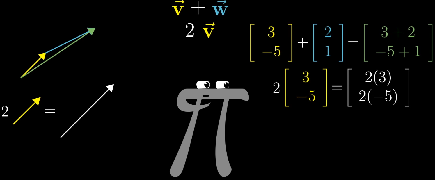
- 物理直观:首尾相连法则。若有向量v ⃗ = [ 3 − 5 ] \vec {v} = \begin {bmatrix} 3 \\ -5 \end {bmatrix}v=[3−5] 与 w ⃗ = [ 2 1 ] \vec {w} = \begin {bmatrix} 2 \\ 1 \end {bmatrix}w=[21],将 w ⃗ \vec {w}w 的起点与 v ⃗ \vec {v}v的终点重合,从v ⃗ \vec {v}v 起点指向 w ⃗ \vec {w}w终点的向量即为v ⃗ + w ⃗ \vec {v} + \vec {w}v+w。
- 代数计算:坐标对应相加,即v ⃗ + w ⃗ = [ 3 + 2 − 5 + 1 ] = [ 5 − 4 ] \vec {v} + \vec {w} = \begin {bmatrix} 3 + 2 \\ -5 + 1 \end {bmatrix} = \begin {bmatrix} 5 \\ -4 \end {bmatrix}v+w=[3+2−5+1]=[5−4]。
1.2.2 向量数乘
- 物理直观:缩放执行。若有标量k = 2 k = 2k=2 与向量 v ⃗ = [ 3 − 5 ] \vec {v} = \begin {bmatrix} 3 \\ -5 \end {bmatrix}v=[3−5],数乘结果为向量长度变为原来的2 22倍,方向与原向量一致(k > 0 k>0k>0)或相反(k < 0 k<0k<0)。
- 代数计算:坐标与标量分别相乘,即k v ⃗ = 2 × [ 3 − 5 ] = [ 6 − 10 ] k\vec {v} = 2 \times \begin {bmatrix} 3 \\ -5 \end {bmatrix} = \begin {bmatrix} 6 \\ -10 \end {bmatrix}kv=2×[3−5]=[6−10]。
1.3 坐标系:向量的统一表示
借助引入坐标系(如笛卡尔坐标系),可将物理视角的 “箭头” 与计算机视角的 “数字列表” 统一:
- 以坐标原点为向量的起点,坐标值的正负表示方向(如x xx轴正方向为右,负方向为左);
- 任意向量可表示为[ x y ] \begin {bmatrix} x \\ y \end {bmatrix}[xy](二维)或 [ x y z ] \begin {bmatrix} x \\ y \\ z \end {bmatrix}xyz(三维),其中x , y , z x,y,zx,y,z为向量在各坐标轴上的投影长度。
2 线性组合、张成空间与基
Mathematics requires a small dose, not of genius, but of an imaginative freedom which, in a larger dose, would be insanity - Angus K. Rodgers
少量的自由想象,但想象太过自由又会陷入疯狂 ——安古斯·罗杰斯就是数学需要的不是天赋,而
2.1 线性组合
给定两个非共线的非零向量v ⃗ \vec {v}v 与 w ⃗ \vec {w}w,对于任意标量a , b a,ba,b,表达式 a v ⃗ + b w ⃗ a\vec {v} + b\vec {w}av+bw 称为 v ⃗ \vec {v}v 与 w ⃗ \vec {w}w 的线性组合。
- 几何直观:固定一个标量(如a aa),让另一个标量(如b bb)自由变化,线性组合的终点会形成一条直线;若两个标量均自由变化,终点会覆盖整个二维平面(非共线时)。
2.2 张成的空间(Span)
所有可由给定向量的线性组合表示的向量集合,称为这些向量张成的空间。
- 二维空间中,若v ⃗ \vec {v}v 与 w ⃗ \vec {w}w共线,其张成的空间是一条直线;若不共线,张成的空间是整个二维平面;
- 三维空间中,若三个向量共面,其张成的空间是一个平面;若不共面,张成的空间是整个三维空间。
2.3 基(Basis)
张成向量空间的线性无关向量组描述空间的 “基本单位”。就是称为该空间的一组基,基
- 笛卡尔坐标系的标准基为{ ı ^ , ȷ ^ } \{\hat {\imath}, \hat {\jmath}\}{^,^}(二维)或 { ı ^ , ȷ ^ , k ^ } \{\hat {\imath}, \hat {\jmath}, \hat {k}\}{^,^,k^}(三维),其中ı ^ = [ 1 0 ] \hat {\imath} = \begin {bmatrix} 1 \\ 0 \end {bmatrix}^=[10],ȷ ^ = [ 0 1 ] \hat {\jmath} = \begin {bmatrix} 0 \\ 1 \end {bmatrix}^=[01],k ^ = [ 0 0 1 ] \hat {k} = \begin {bmatrix} 0 \\ 0 \\ 1 \end {bmatrix}k^=001(单位向量);
- 任意向量可由基的线性组合表示,如二维向量[ x y ] = x ı ^ + y ȷ ^ \begin {bmatrix} x \\ y \end {bmatrix} = x\hat {\imath} + y\hat {\jmath}[xy]=x^+y^。
2.4 线性相关与线性无关
- 线性相关:若存在不全为0 00 的标量 a 1 , a 2 , ⋯ , a n a_1,a_2,\cdots,a_na1,a2,⋯,an,使得 a 1 v 1 ⃗ + a 2 v 2 ⃗ + ⋯ + a n v n ⃗ = 0 ⃗ a_1\vec {v_1} + a_2\vec {v_2} + \cdots + a_n\vec {v_n} = \vec {0}a1v1+a2v2+⋯+anvn=0,则称向量组{ v 1 ⃗ , v 2 ⃗ , ⋯ , v n ⃗ } \{\vec {v_1},\vec {v_2},\cdots,\vec {v_n}\}{v1,v2,⋯,vn}线性相关。几何上表现为向量共线(二维)或共面(三维),即移除一个向量后张成的空间不变(存在冗余)。
- 线性无关:若仅当 a 1 = a 2 = ⋯ = a n = 0 a_1 = a_2 = \cdots = a_n = 0a1=a2=⋯=an=0 时,a 1 v 1 ⃗ + ⋯ + a n v n ⃗ = 0 ⃗ a_1\vec {v_1} + \cdots + a_n\vec {v_n} = \vec {0}a1v1+⋯+anvn=0成立,则称向量组线性无关。几何上表现为向量不共线(二维)或不共面(三维),无冗余向量。
基的严格定义:向量空间的一组基是 “张成该空间的线性无关向量集”,基向量的个数等于空间的维度。
3 矩阵与线性变换
Unfortunately, no one can be told what the Matrix is. You have to see it yourself -Morpheus
很遗憾,Matrix(矩阵)是什么是说不清的。你必须得自己亲眼看看 ——墨菲斯
3.1 变换的本质
“变换” 是 “函数” 的几何化表述:函数接受输入值并输出结果,而变换接受输入向量并输出变换后的向量(记为L ( v ⃗ ) L (\vec {v})L(v),其中 L LL表示变换)。

与普通函数不同,“变换” 强调用运动视角理解向量的映射关系,例如 “旋转”“剪切”“缩放” 等操作均可视为对向量的变换,且可通过可视化直观呈现。
3.2 线性变换的定义与性质
满足特定条件的变换被称为线性变换,其核心定义、几何性质及相关扩展概念如下。
3.2.1 线性变换的定义
线性变换需同时满足以下两个本质条件,这是判断一个变换是否为线性变换的核心依据:
- 直线保持性:变换后直线仍为直线,不会发生弯曲变形;
- 原点固定性:变换前后坐标原点的位置保持不变,即原点映射到自身。
3.2.2 线性变换的几何性质
从几何直观角度分析,线性变换具有以下三个关键性质,可进一步解释其对空间图形的作用规律:
- 直线映射为直线:该性质是“直线保持性”的几何体现,线性变换不会将直线扭曲为曲线,仅改变直线的位置、方向或长度(非弯曲);
- 原点保持固定:与定义中的“原点固定性”一致,线性变换始终将坐标原点( 0 , 0 ) (0,0)(0,0)(或高维空间原点)映射到自身,不会产生原点的平移;
- 网格线保持平行:若空间中存在由平行直线构成的网格(如平面直角坐标系的网格线),线性变换后网格线的平行关系不会被破坏,仍保持相互平行。
3.2.3 网格线的等距分布特性
线性变换虽能保持网格线的平行性,但不必然保持网格线的等距分布(即网格线间的间距可能改变)。仅在特定类型的线性变换下,网格线才会维持等距分布,具体示例如下:
| 线性变换类型 | 网格线等距分布情况 | 说明 |
|---|---|---|
| 均匀缩放 | 保持等距 | 对图形沿各坐标轴按相同比例缩放,网格线间距同比例变化,仍保持均匀; |
| 旋转 | 保持等距 | 图形绕原点旋转时,网格线仅方向改变,间距始终不变; |
| 剪切变换 | 不保持等距 | 图形沿某一方向“剪切”变形,网格线虽仍平行,但间距发生非均匀变化。 |
(图示:线性变换对网格线的影响,以剪切变换为例,网格线平行但间距改变)
3.2.4 线性变换的等价代数性质
从代数角度看,线性变换的定义可等价表述为满足“可加性”与“数乘性”,这是线性代数中描述线性变换的标准形式。
设 L LL为线性变换,v ⃗ \vec{v}v、w ⃗ \vec{w}w为任意向量,c cc为任意标量,则:
- 可加性:L ( v ⃗ + w ⃗ ) = L ( v ⃗ ) + L ( w ⃗ ) L(\vec{v} + \vec{w}) = L(\vec{v}) + L(\vec{w})L(v+w)=L(v)+L(w),即两个向量和的变换等于两个向量变换的和;
- 数乘性:L ( c v ⃗ ) = c L ( v ⃗ ) L(c\vec{v}) = cL(\vec{v})L(cv)=cL(v),即一个向量与标量乘积的变换等于该向量变换与标量的乘积。
3.2.5 相关扩展概念:仿射变换
若一个变换仅满足“直线保持性”,但不满足“原点固定性”(即变换后原点位置发生移动),则该变换称为仿射变换(Affine Transformation)。
仿射变换的代数表达式为:y ⃗ = A x ⃗ + b ⃗ \vec{y} = A\vec{x} + \vec{b}y=Ax+b(其中 b ⃗ ≠ 0 ⃗ \vec{b} \neq \vec{0}b=0),可理解为“线性变换与平移变换的结合”——式中A x ⃗ A\vec{x}Ax代表线性变换部分,b ⃗ \vec{b}b代表平移变换部分(b ⃗ ≠ 0 ⃗ \vec{b} \neq \vec{0}b=0确保存在平移,原点发生移动)。
3.3 矩阵:线性变换的数字描述
“基向量的变换”—— 由于任意向量可由基的线性组合表示,只要确定基向量变换后的位置,即可确定整个空间的变换。就是线性变换的关键
3.3.1 矩阵的构造
以二维空间的标准基{ ı ^ , ȷ ^ } \{\hat {\imath}, \hat {\jmath}\}{^,^} 为例:
- 设 ı ^ \hat {\imath}^ 变换后为 ı ′ ⃗ = [ a c ] \vec {\imath'} = \begin {bmatrix} a \\ c \end {bmatrix}′=[ac],ȷ ^ \hat {\jmath}^ 变换后为 ȷ ′ ⃗ = [ b d ] \vec {\jmath'} = \begin {bmatrix} b \\ d \end {bmatrix}′=[bd];
- 将 ı ′ ⃗ \vec {\imath'}′作为第一列、ȷ ′ ⃗ \vec {\jmath'}′作为第二列,构成矩阵A = [ a b c d ] A = \begin {bmatrix} a & b \\ c & d \end {bmatrix}A=[acbd],该矩阵即为线性变换的数字描述。
3.3.2 矩阵与向量的乘法
对于任意向量x ⃗ = [ x y ] \vec {x} = \begin {bmatrix} x \\ y \end {bmatrix}x=[xy],其变换后的结果y ⃗ = A x ⃗ \vec {y} = A\vec {x}y=Ax可通过以下步骤计算:
将 x ⃗ \vec {x}x分解为基的线性组合:x ⃗ = x ı ^ + y ȷ ^ \vec {x} = x\hat {\imath} + y\hat {\jmath}x=x^+y^;
对基向量应用线性变换:L ( x ⃗ ) = x L ( ı ^ ) + y L ( ȷ ^ ) = x ı ′ ⃗ + y ȷ ′ ⃗ L (\vec {x}) = xL (\hat {\imath}) + yL (\hat {\jmath}) = x\vec {\imath'} + y\vec {\jmath'}L(x)=xL(^)+yL(^)=x′+y′;
代入基向量变换结果,得到代数表达式:
A x ⃗ = [ a b c d ] [ x y ] = x [ a c ] + y [ b d ] ⏟ 直观的部分 = [ a x + b y c x + d y ] A\vec {x} = \begin{bmatrix}\textcolor{green}{a} & \textcolor{red}{b} \\\textcolor{green}{c} & \textcolor{red}{d}\end{bmatrix}\begin{bmatrix}x \\y\end{bmatrix}=\underbrace{x\begin{bmatrix}\textcolor{green}{a} \\\textcolor{green}{c}\end{bmatrix}+y\begin{bmatrix}\textcolor{red}{b} \\\textcolor{red}{d}\end{bmatrix}}_{\text{直观的部分}}=\begin{bmatrix}\textcolor{green}{a}x + \textcolor{red}{b}y \\\textcolor{green}{c}x + \textcolor{red}{d}y\end{bmatrix}Ax=[acbd][xy]=直观的部分x[ac]+y[bd]=[ax+bycx+dy]其中绿色元素代表单位向量i ^ \hat{i}i^经变换后的向量,红色元素代表单位向量j ^ \hat{j}j^经变换后的向量。
上述公式即为矩阵乘法公式。
示例:若变换矩阵A
=
[
3
1
1
2
]
A = \begin {bmatrix} 3 & 1 \\ 1 & 2 \end {bmatrix}A=[3112](ı
^
\hat {\imath}^→[
3
1
]
\begin {bmatrix} 3 \\ 1 \end {bmatrix}[31],ȷ
^
\hat {\jmath}^→[
1
2
]
\begin {bmatrix} 1 \\ 2 \end {bmatrix}[12]),向量 x
⃗
=
[
−
1
2
]
\vec {x} = \begin {bmatrix} -1 \\ 2 \end {bmatrix}x=[−12]的变换结果为:
A
x
⃗
=
(
−
1
)
×
[
3
1
]
+
2
×
[
1
2
]
=
[
−
3
+
2
−
1
+
4
]
=
[
−
1
3
]
A\vec {x} = (-1)\times\begin {bmatrix} 3 \\ 1 \end {bmatrix} + 2\times\begin {bmatrix} 1 \\ 2 \end {bmatrix} = \begin {bmatrix} -3 + 2 \\ -1 + 4 \end {bmatrix} = \begin {bmatrix} -1 \\ 3 \end {bmatrix}Ax=(−1)×[31]+2×[12]=[−3+2−1+4]=[−13]
线性变换步骤
Step 1: 移动x xx 轴
绿色单位向量i ^ \hat{i}i^(x xx轴)进行移动(变换)。Step 2: 移动y yy 轴
红色单位向量j ^ \hat{j}j^(y yy轴)进行移动(变换)。Step 3: 向量乘法 -x xx 轴坐标
目标向量的 x xx轴坐标值与变换后的i ^ \hat{i}i^向量进行向量乘法。Step 4: 向量乘法 -y yy 轴坐标
目标向量的 y yy轴坐标值与变换后的j ^ \hat{j}j^向量进行向量乘法。Step 5: 向量加法
将步骤 3 和步骤 4 得到的向量进行向量加法,得到最终的线性变换结果。
4 矩阵乘法与线性变换复合
It is my experience that proofs involving matrices can be shortened by 50% if one throws the matrices out -Emil Artin
据我的经验,如果丢掉矩阵的话,那些涉及矩阵的证明能够缩短一半 ——埃米尔·阿廷
4.1 复合变换的概念
在数学领域,向量变换可通过矩阵乘法达成。
若向量先经旋转(保持单位向量i ^ \hat {i}i^不变,矩阵第一列为 (1,0))、再经剪切(将单位向量j ^ \hat {j}j^移至 (1,1)),总变换矩阵可由旋转矩阵与剪切矩阵相乘得到,这一过程即矩阵乘法。
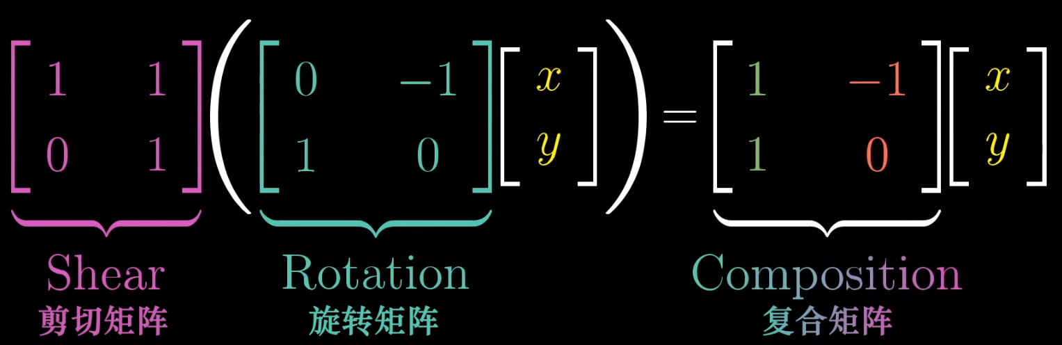
向量连续应用多个线性变换(如先旋转再剪切)的组合,称为复合变换,对应的矩阵称为复合矩阵。
矩阵乘法的变换顺序
设第一个变换的矩阵为M 1 M_1M1(如旋转变换),第二个变换的矩阵为M 2 M_2M2(如剪切变换),则向量x ⃗ \vec {x}x经过复合变换后的结果为M 2 ( M 1 x ⃗ ) M_2 (M_1\vec {x})M2(M1x),复合矩阵记为M = M 2 M 1 M = M_2M_1M=M2M1。
注意:变换顺序为 “从右向左”,与函数复合f ( g ( x ) ) f (g (x))f(g(x)) 一致。
4.2 矩阵乘法的几何意义
“基向量的二次变换”,计算复合矩阵就是矩阵乘法的本质M = M 2 M 1 M = M_2M_1M=M2M1的步骤如下:
取 M 1 M_1M1的第一列(即ı ^ \hat {\imath}^ 经 M 1 M_1M1变换后的向量ı 1 ⃗ \vec {\imath_1}1),将其作为输入向量应用M 2 M_2M2 变换,得到 ı 2 ⃗ = M 2 ı 1 ⃗ \vec {\imath_2} = M_2\vec {\imath_1}2=M21,此为 M MM 的第一列;
取 M 1 M_1M1的第二列(即ȷ ^ \hat {\jmath}^ 经 M 1 M_1M1变换后的向量ȷ 1 ⃗ \vec {\jmath_1}1),将其作为输入向量应用M 2 M_2M2 变换,得到 ȷ 2 ⃗ = M 2 ȷ 1 ⃗ \vec {\jmath_2} = M_2\vec {\jmath_1}2=M21,此为 M MM 的第二列;
复合矩阵 M = [ ı 2 ⃗ ȷ 2 ⃗ ] M = \begin {bmatrix} \vec {\imath_2} & \vec {\jmath_2} \end {bmatrix}M=[22]。
示例:设 M 1 = [ cos θ − sin θ sin θ cos θ ] M_1 = \begin {bmatrix} \cos\theta & -\sin\theta \\ \sin\theta & \cos\theta \end {bmatrix}M1=[cosθsinθ−sinθcosθ](旋转变换),M 2 = [ 1 1 0 1 ] M_2 = \begin {bmatrix} 1 & 1 \\ 0 & 1 \end {bmatrix}M2=[1011](剪切变换,ı ^ \hat {\imath}^ 不变,ȷ ^ \hat {\jmath}^→[ 1 1 ] \begin {bmatrix} 1 \\ 1 \end {bmatrix}[11]),则复合矩阵M = M 2 M 1 M = M_2M_1M=M2M1 的
第一列为
M 2 × [ cos θ sin θ ] = [ cos θ + sin θ sin θ ] M_2\times\begin {bmatrix} \cos\theta \\ \sin\theta \end {bmatrix} = \begin {bmatrix} \cos\theta + \sin\theta \\ \sin\theta \end {bmatrix}M2×[cosθsinθ]=[cosθ+sinθsinθ],
第二列为
M 2 × [ − sin θ cos θ ] = [ − sin θ + cos θ cos θ ] M_2\times\begin {bmatrix} -\sin\theta \\ \cos\theta \end {bmatrix} = \begin {bmatrix} -\sin\theta + \cos\theta \\ \cos\theta \end {bmatrix}M2×[−sinθcosθ]=[−sinθ+cosθcosθ],
即:
M = [ cos θ + sin θ cos θ − sin θ sin θ cos θ ] M = \begin {bmatrix} \cos\theta + \sin\theta & \cos\theta - \sin\theta \\ \sin\theta & \cos\theta \end {bmatrix}M=[cosθ+sinθsinθcosθ−sinθcosθ]
4.3 矩阵乘法的性质
通过几何直观可快速验证矩阵乘法的性质:
- 不满足交换律:M 2 M 1 ≠ M 1 M 2 M_2M_1 \neq M_1M_2M2M1=M1M2(先旋转再剪切,与先剪切再旋转的结果不同);
- 满足结合律:( M 3 M 2 ) M 1 = M 3 ( M 2 M 1 ) (M_3M_2) M_1 = M_3 (M_2M_1)(M3M2)M1=M3(M2M1)(三次变换的顺序固定,分组不影响结果)。
4.4 高维扩展
三维空间的线性变换可由3 × 3 3 \times 33×3矩阵描述,矩阵的列对应标准基{ ı ^ , ȷ ^ , k ^ } \{\hat {\imath}, \hat {\jmath}, \hat {k}\}{^,^,k^}变换后的向量。工程中(如机器人运动控制、3D 建模),3 × 3 3 \times 33×3矩阵可精确描述三维空间的旋转、缩放等操作,是连接数字计算与物理运动的重要软件。
- 线性代数 | 要义 / 本质 (下篇)-CSDN博客
https://blog.csdn.net/u013669912/article/details/153215664
via:
Essence of linear algebra • Evan Jonokuchi
https://ejonokuchi.com/essence.htmlthe excellent YouTube series
https://www.youtube.com/playlist?list=PLZHQObOWTQDPD3MizzM2xVFitgF8hE_ab【直观详解】线性代数的本质 | Go Further | Stay Hungry, Stay Foolish
https://charlesliuyx.github.io/2017/10/06/【直观详解】线性代数的本质/

 浙公网安备 33010602011771号