Pytorch 2.3.5 预备知识 Pytorch下的概率论

我很喜欢的一句话 “在某种形式上，机器学习就是做出预测。” 突出了概率论于机器学习的重要性。

Pytorch官方是这样描述 torch.distributions 这个方法模块的：

The distributions package contains parameterizable(可参数化的) probability distributions and sampling functions(抽样函数，暂时未学到). This allows the construction(构造) of stochastic(随机的) computation graphs(计算图) and stochastic gradient estimators(随机梯度计算器) for optimization(优化). This package generally follows the design of the TensorFlow Distributions package.(按照TensorFlow的标准来写的)。

It is not possible to directly backpropagate through random samples. However, there are two main methods for creating surrogate functions that can be backpropagated through. These are the score function estimator/likelihood ratio estimator/REINFORCE and the pathwise derivative estimator. REINFORCE is commonly seen as the basis for policy gradient methods in reinforcement learning, and the pathwise derivative estimator is commonly seen in the reparameterization trick in variational autoencoders. Whilst the score function only requires the value of samples f(x)f(x), the pathwise derivative requires the derivative \(f'(x)\) . The next sections discuss these two in a reinforcement learning example. For more details see Gradient Estimation Using Stochastic Computation Graphs . 不可能通过随机样本直接反向传播。 但是，有两种主要方法可以创建可以反向传播的代理函数。 这些是分数函数估计量/似然比估计量/REINFORCE和路径导数估计量。 在强化学习中，REINFORCE通常被看作是政策梯度方法的基础，而路径导数估计通常出现在变分自编码器的重参数化技巧中。 虽然评分函数只需要样本\(f(x)\)的值，但路径导数需要导数\(f'(x)\)。 下一节将在一个强化学习示例中讨论这两种方法。 要了解更多细节，请参见使用随机计算图的梯度估计。

预备知识 Pytorch下的概率论 基础知识点击这里

torch.distributions.multinomial.Multinomial(input, num_samples,replacement=False, out=None)

input:vector in vector out ，matrix in and matrix out
num_samples: 采样的次数
replacement :默认值值是False(即不放回采样)

具体的使用方式：

fair_probs = torch.ones([6])/6
td.multinomial.Multinomial(10000,fair_probs).sample() #它在索引 𝑖 处的值是采样结果中 𝑖 出现的次数。

对于上面的一小段的简短代码，可以这样子来理解：1️⃣先生成一个概率张量 \(\vec{a}\) 2️⃣ 将这个\(\vec{a}\)传入Multinomial(每次抽样个数[一个样本的数量]，传入的\(\vec{a}\))方法中，而上面的代码你可以理解fair_probs 为一个骰子的每个点的概率的张量，传入Mutinomial()中生成样本。

因为我们是从一个公平的骰子中生成的数据，我们知道每个结果都有真实的概率\(\frac{1}{6}\)，大约是\(0.167\)，所以上面输出的估计值看起来不错。我们也可以看到这些概率如何随着时间的推移收敛到真实概率。让我们进行500组实验，每组抽取10个样本。

import torch,torch.distributions.multinomial as multinomial 
import matplotlib.pyplot as plt 
import numpy as np,numpy 

counts = td.multinomial.Multinomial(10,fair_probs).sample((500,)) 
#这里暂且理解为sample需要传入一个可迭代对象，但是目前我们只需要传入一个抽样次数参数，
#抽样次数很明显是一个int，非可迭代对象，因此我们创建一个元组(500,)可迭代对象
cum_counts = counts.cumsum(dim=0)  # cumsum是从MATLAB中引申过来的一个函数，作用是计算累加值
estimates = cum_counts / cum_counts.sum(dim=1, keepdims=True) # 行向量求和  归一化  

print(estimates)

for i in range(6): 
    plt.plot(estimates[:, i].numpy(), label=("P(die=" + str(i + 1) + ")"))
    plt.gca().set_xlabel("实验估计")
    plt.gca().set_ylabel("估算概率")
    plt.legend()

输出:

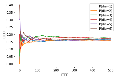
注意！！如果matplotlib还是不是很熟悉的同学建议看看我的另外一文章Matplot基本用法+常识，我这里没有显示中文的原因是我没有导入中文字体库，而matplotlib是默认不支持中文的

一点小小的提示：torch.sum(dim=1,keepdims=True) 和torch.cumsum(dim=1)是不同的，具体差异如下：
输入：

a = torch.arange(12).reshape(3,4) 
sum_a0 = a.sum(dim=0,)
a,sum_a0 

输出：

         [ 4,  5,  6,  7],
         [ 8,  9, 10, 11]]),
 tensor([[12, 15, 18, 21]]))

keepdims=True 和 cumsum() 最大的区别就是，前者只是简单求和然后保留维度，也就是框框[][]，但是后者是累计求和

🔺🔺🔺此文还在编辑中，如果有任何错误请指出。🔺🔺🔺