零售行业下MongoDB在产品目录系统、库存系统、个性推荐系统中的应用【转载】

Retail Reference Architecture Part 1: Building a Flexible, Searchable, Low-Latency Product Catalog

Product catalog data management is a complex problem for retailers today. After years of relying on multiple monolithic, vendor-provided systems, retailers are now reconsidering their options and looking to the future.

In today’s vendor-provided systems, product data must frequently be moved back and forth using ETL processes to ensure all systems are operating on the same data set. This approach is slow, error prone, and expensive in terms of development and management. In response, retailers are now making data services available individually as part of a centralized service-oriented architecture (SOA).

This is a pattern that we commonly see at MongoDB, so much so that we’ve begun to define some best practices and reference architecture specifically targeted at the retail space. As part of that effort, today we’ll be taking a look at implementing a catalog service using MongoDB as the first of a three part series on retail architecture.

Why MongoDB?

Many different database types are able to fulfill our product catalog use case, so why choose MongoDB?

• Document flexibility: Each MongoDB document can store data represented as rich JSON structures. This makes MongoDB ideal for storing just about anything, including very large catalogs with thousands of variants per item.

• Dynamic schema: JSON structures within each document can be altered at any time, allowing for increased agility and easy restructuring of data when needs change. In MongoDB, these multiple schemas can be stored within a single collection and can use shared indexes, allowing for efficient searching of both old and new formats simultaneously.

• Expressive query language: The ability to perform queries across many document attributes simplifies many tasks. This can also improve application performance by lowering the required number of database requests.

• Indexing: Powerful secondary, compound and geo-indexing options are available in MongoDB right out of the box, quickly enabling features like sorting and location-based queries.

• Data consistency: By default, all reads and writes are sent to the primary member of a MongoDB replica set. This ensures strong consistency, an important feature for retailers, who may have many customers making requests against the same item inventory.

• Geo-distributed replicas: Network latency due to geographic distance between a data source and the client can be problematic, particularly for a catalog service which would be expected to sustain a large number of low-latency reads. MongoDB replica sets can be geo-distributed, so that they are close to users for fast access, mitigating the need for CDNs in many cases.

These are just a few of the characteristics of MongoDB that make it a great option for retailers. Next, we’ll take a look at some of the specifics of how we put some of these to use in our retail reference architecture to support a number of features, including:

• Searching for items and item variants
• Retrieving per store pricing for items
• Enabling catalog browsing with faceted search

Item Data Model

The first thing we need to consider is the data model for our items. In the following examples we are showing only the most important information about each item, such as category, brand and description:

{
	“_id”: “30671”, //main item ID
	“department”: “Shoes”,
	“category”: “Shoes/Women/Pumps”,
	“brand”: “Calvin Klein”,
	“thumbnail”: “http://cdn.../pump.jpg”,
	“title”: “Evening Platform Pumps”,
	“description”: “Perfect for a casual night out or a formal event.”,
	“style”: “Designer”,
	…
}

This type of simple data model allows us to easily query for items based on the most demanded criteria. For example, using db.collection.findOne, which will return a single document that satisfies a query:

• Get item by ID 
  db.definition.findOne({_id:”301671”})

• Get items for a set of product IDs 
  db.definition.findOne({_id:{$in:[”301671”,”452318”]}})

• Get items by category prefix 
  db.definition.findOne({category:/^Shoes\/Women/})

Notice how the second and third queries used the $in operator and a regular expression, respectively. When performed on properly indexed documents, MongoDB is able to provide high throughput and low latency for these types of queries.

Variant Data Model

Another important consideration for our the product catalog is item variants, such as available sizes, colors, and styles. Our item data model above only captures a small amount of the data about each catalog item. So what about all of the available item variations we may need to retrieve, such as size and color?

One option is to store an item and all its variants together in a single document. This approach has the advantage of being able to retrieve an item and all variants in a single query. However, it is not the best approach in all cases. It is an important best practice to avoid unbounded document growth. If the number of variants and their associated data is small, it may make sense to store them in the item document.

Another option is to create a separate variant data model that can be referenced relative to the primary item:

{
	“_id”: ”93284847362823”, //variant sku
	“itemId”: “30671”, //references the main item
	“size”: 6.0,
	“color”: “red”
	…
}

This data model allows us to do fast lookups of specific item variants by their SKU number:

db.variation.find({_id:”93284847362823”})

As well as all variants for a specific item by querying on the itemId attribute:

db.variation.find({itemId:”30671”}).sort({_id:1})

In this way, we maintain fast queries on both our primary item for displaying in our catalog, as well as every variant for when the user requests a more specific product view. We also ensure a predictable size for the item and variant documents.

Per Store Pricing

Another consideration when defining the reference architecture for our product catalog is pricing. We’ve now seen a few ways that the data model for our items can be structured to quickly retrieve items directly or based on specific attributes. Prices can vary by many factors, like store location. We need a way to quickly retrieve the specific price of any given item or item variant. This can be very problematic for large retailers, since a catalog with a million items and one thousand stores means we must query across a collection of a billion documents to find the price of any given item.

We could, of course, store the price for each variant as a nested document within the item document, but a better solution is to again take advantage of how quickly MongoDB is able to query on _id. For example, if each item in our catalog is referenced by an itemId, while each variant is referenced by a SKU number, we can set the _id of each document to be a concatenation of the itemId or SKU and the storeId associated with that price variant. Using this model, the _id for the pair of pumps and its red variant described above would look something like this:

• Item: 30671_store23
• Variant: 93284847362823_store23

This approach also provides a lot of flexibility for handling pricing, as it allows us to price items at the item or the variant level. We can then query for all prices or just the price for a particular location:

• All prices: db.prices.find({_id:/^30671/})
• Store price: db.prices.find({_id:/^30671_store23/})

We could even add other combinations, such as pricing per store group, and get all possible prices for an item with a single query by using the $in operator:

db.prices.find({_id:{$in:[	“30671_store23”,
				“30671_sgroup12”,
				“93284847362823_store23”,
				“93284847362823_sgroup12” ]}})

Browse and Search Products

The biggest challenge for our product catalog is to enable browsing with faceted search. While many users will want to search our product catalog for a specific item or criteria they are looking for, many others will want to browse, then narrow the returned results by any number of attributes. So given the need to create a page like this:

We have many challenges:

• Response time: As the user browses, each page of results should return in milliseconds.
• Multiple attributes: As the user selects different facets—e.g. brand, size, color—new queries must be run on multiple document attributes.
• Variant-level attributes: Some user-selected attributes will be queried at the item level, such as brand, while others will be at the variant level, such as size.
• Multiple variants: Thousands of variants can exist for each item, but we only want to display each item once, so results must be de-duplicated.
• Sorting: The user needs to be allowed to sort on multiple attributes, like price and size, and that sorting operation must perform efficiently.
• Pagination: Only a small number of results should be returned per page, which requires deterministic ordering.

Many retailers may want to use a dedicated search engine as the basis of these features. MongoDB provides an open source connector project, which allows the use of Apache Solr and Elasticsearch with MongoDB. For our reference architecture, however, we wanted to implement faceted search entirely within MongoDB.

To accomplish this, we create another collection that stores what we will call summary documents. These documents contain all of the information we need to do fast lookups of items in our catalog based on various search facets.

{ 
	“_id”: “30671”,
	“title”: “Evening Platform Pumps”,
	“department”: “Shoes”,
	“Category”: “Women/Shoes/Pumps”,
   	“price”: 149.95,
	“attrs”: [“brand”: “Calvin Klein”, …],
	“sattrs”: [“style”: ”Designer”, …],
	“vars”: [
		{
			“sku”: “93284847362823”,
			“attrs”: [{“size”: 6.0}, {“color”: “red”}, …],
			“sattrs”: [{“width”: 8.0}, {“heelHeight”: 5.0}, …],
		}, … //Many more SKUs
	]
<p>}

 

Note that in this data model we are defining attributes and secondary attributes. While a user may want to be able to search on many different attributes of an item or item variant, there is only a core set that are most frequently used. For example, given a pair of shoes, it may be more common for a user to filter their search based on available size than filtering by heel height. By using both the attrand sattr attributes in our data model, we are able to make all of these item attributes available to search, but incur only the expense of indexing the most used attributes by indexing only attr.

Using this data model, we would create compound indices on the following combinations:

• department + attr + category + _id
• department + vars.attr + category + _id
• department + category + _id
• department + price + _id
• department + rating + _id

In these indices, we always start with department, and we assume users will chose the department to refine their search results. For a catalog without departments, we could have just as easily begun with another common facet like category or type. We can then perform the queries needed for faceted search and quickly return the results to the page:

• Get summary from itemId 
  db.variation.find({_id:”30671”})

• Get summary of specific item variant 
  db.variation.find({vars.sku:”93284847362823”},{“vars.$”:1})

• Get summaries for all items by department 
  db.variation.find({department:”Shoes”})

• Get summaries with a mix of parameters
  db.variation.find({ “department”:”Shoes”,
        “vars.attr”: {“color”:”red”},
        “category”: “^/Shoes/Women”})

Recap

We’ve looked at some best practices for modeling and indexing data for a product catalog that supports a variety of application features, including item and item variant lookup, store pricing, and catalog browsing using faceted search. Using these approaches as a starting point can help you find the best design for your own implementation.

Learn more

To discover how you can re-imagine the retail experience with MongoDB, read our white paper. In this paper, you'll learn about the new retail challenges and how MongoDB addresses them.

 

转载于 《https://www.mongodb.com/blog/post/retail-reference-architecture-part-1-building-flexible-searchable-low-latency-product》

 

Retail Reference Architecture Part 2: Approaches to Inventory Optimization

In part one of our series on retail reference architecture we looked at some best practices for how a high-volume retailer might use MongoDB as the persistence layer for a large product catalog. This involved index, schema, and query optimization to ensure our catalog could support features like search, per-store pricing and browsing with faceted search in a highly performant manner. Over the next two posts we will be looking at approaches to similar types of optimization, but applied to an entirely different aspect of retail business, inventory.

A solid central inventory system that is accessible across a retailer’s stores and applications is a large part of the foundation needed for improving and enriching the customer experience. Here are just a few of the features that a retailer might want to enable:

• Reliably check real-time product availability.
• Give the option for in-store pick-up at a particular location.
• Detect the need for intra-day replenishment if there is a run on an item.

The Problem with Inventory Systems

These are features that seem basic but they present real challenges given the types of legacy inventory systems commonly used by major retailers. In these systems, individual stores keep their own field inventories, which then report data back to the central RDBMS at a set time interval, usually nightly. That RDBMS then reconciles and categorizes all of the data received that day and makes it available for operations like analytics, reporting, as well as consumption by external and internal applications. Commonly there is also a caching layer present between the RDBMS and any applications, as relational databases are often not well-suited to the transaction volume required by such clients, particularly if we are talking about a consumer-facing mobile or web app.

So the problem with the status quo is pretty clear. The basic setup of these systems isn’t suited to providing a continually accurate snapshot of how much inventory we have and where that inventory is located. In addition, we also have the increased complexity involved in maintaining multiple systems, i.e. caching, persistence, etc. MongoDB, however, is ideal for supporting these features with a high degree of accuracy and availability, even if our individual retail stores are very geographically dispersed.

Design Principles

To begin, we determined that the inventory system in our retail reference architecture needed to do the following:

• Provide a single view of inventory, accessible by any client at any time.
• Be usable by any system that needs inventory data.
• Handle a high-volume, read-dominated workload, i.e. inventory checks.
• Handle a high volume of real-time writes, i.e. inventory updates.
• Support bulk writes to refresh the system of record.
• Be geographically distributed.
• Remain horizontally scalable as the number of stores or items in inventory grows.

In short, what we needed was to build a high performance, horizontally scalable system where stores and clients over a large geographic area could transact in real-time with MongoDB to view and update inventory.

Stores Schema

Since a primary requirement of our use case was to maintain a centralized, real-time view of total inventory per store, we first needed to create the schema for a stores collection so that we had locations to associate our inventory with. The result is a fairly straightforward document per store:

{
	“_id”:ObjectId(“78s89453d8chw28h428f2423”),
	“className”:”catalog.Store”,
	“storeId”:”store100”,
	“name”:”Bessemer Store”,
	“address”:{
		“addr1”:”1 Main St.”,
		“city”:”Bessemer”,
		“state”:”AL”,
		“zip”:”12345”,
		“country”:”USA”
	},
	“location”:[-86.95444, 33.40178],
	…
}

We then created the following indices to optimize the most common types of reads on our store data:

• {“storeId”:1},{“unique”:true}: Get inventory for a specific store.
• {“name”:1}: Get a store by name.
• {“address.zip”:1}: Get all stores within a zip code, i.e. store locator.
• {“location”: 2dsphere}: Get all stores around a specified geolocation.

Of these, the location index is especially useful for our purposes, as it allows us to query stores by proximity to a location, e.g. a user looking for the nearest store with a product in stock. To take advantage of this in a sharded environment, we used a geoNear command that retrieves the documents whose ‘location’ attribute is within a specified distance of a given point, sorted nearest first:

db.runCommand({
	geoNear:“stores”,
	near:{
		type:”Point”,
		coordinates:[-82.8006,40.0908], //GeoJSON or coordinate pair
		maxDistance:10000.0, //in meters
		spherical:true //required for 2dsphere indexes
	}
}) 

This schema gave us the ability to locate our objects, but the much bigger challenge was tracking and managing the inventory in those stores.

Inventory Data Model

Now that we had stores to associate our items with, we needed to create an inventory collection to track the actual inventory count of each item and all its variants. Some trade-offs were required for this, however. To both minimize the number of roundtrips to the database, as well as mitigate application-level joins, we decided to duplicate data from the stores collection into the inventory collection. The document we came up with looked like this:

{
	“_id”:”902372093572409542jbf42r2f2432”,
	“storeId”:”store100”,
	“location”:[-86.95444, 33.40178],
	“productId”:”20034”,
	“vars”:[
		{“sku”:”sku1”, “quantity”:”5”},
		{“sku”:”sku2”, “quantity”:”23”},
		{“sku”:”sku3”, “quantity”:”2”},
		…
	]
}

Notice first that we included both the ‘storeId’ and ‘location’ attribute in our inventory document. Clearly the ‘storeId’ is necessary so that we know which store has what items, but what happens when we are querying for inventory near the user? Both the inventory data and store location data are required to complete the request. By adding geolocation data to the inventory document we eliminate the need to execute a separate query to the stores collection, as well as a join between the stores and inventory collections.

For our schema we also decided to represent inventory in our documents at the productId level. As was noted in part one of our retail reference architecture series, each product can have many, even thousands of variants, based on size, color, style, etc., and all these variants must be represented in our inventory. So the question is should we favor larger documents that contain a potentially large variants collection, or many more documents that represent inventory at the variant level? In this case, we favored larger documents to minimize the amount of data duplication, as well as decrease the total number of documents in our inventory collection that would need to be queried or updated.

Next, we created our indices:

• {storeId:1}: Get all items in inventory for a specific store.
• {productId:1},{storeId:1}: Get inventory of a product for a specific store.
• {productId:1},{location:”2dsphere”}: Get all inventory of a product within a specific distance.

It’s worth pointing out here that we chose not to include an index with ‘vars.sku’. The reason for this is that it wouldn’t actually buy us very much, since we are already able to do look ups in our inventory based on ‘productID’. So, for example, a query to get a specific variant sku that looks like this:

db.inventory.find(
	{
		“storeId”:”store100”,
		“productId”:“20034”,
		“vars.sku”:”sku11736”
	},
	{“vars.$”:1}
)

Doesn’t actually benefit much from an added index on ‘vars.sku’. In this case, our index on ‘productId’ is already giving us access to the document, so an index on the variant is unnecessary. In addition, because the variants array can have thousands of entries, an index on it could potentially take up a large block in memory, and consequently decrease the number of documents stored in memory, meaning slower queries. All things considered, an unacceptable trade-off, given our goals.

So what makes this schema so good anyhow? We’ll take a look in our next post at some of the features this approach makes available to our inventory system.

Learn More

To discover how you can re-imagine the retail experience with MongoDB, read our white paper. In this paper, you'll learn about the new retail challenges and how MongoDB addresses them.

 

转载于 《https://www.mongodb.com/blog/post/retail-reference-architecture-part-2-approaches-inventory-optimization》

 

Retail Reference Architecture Part 3: Query Optimization and Scaling

In part one of this series on reference architectures for retail, we discussed how to use MongoDB as the persistence layer for a large product catalog. In part two, we covered the schema and data model for an inventory system. Today we’ll cover how to query and update inventory, plus how to scale the system.

Inventory Updates and Aggregations

At the end of the day, a good inventory system needs to be more than just a system of record for retrieving static data. We also need to be able to perform operations against our inventory, including updates when inventory changes, and aggregations to get a complete view of what inventory is available and where.

The first of these operations, updating the inventory, is both pretty straightforward and nearly as performant as a standard query, meaning our inventory system will be able to handle the high-volume we would expect to receive. To do this with MongoDB we simply retrieve an item by its ‘productId’, then execute an in-place update on the variant we want to update using the $inc operator:

db.inventory.update(
	{
		“storeId”:”store100”,
		“productId”:“20034”,
		“vars.sku”:”sku11736”
	},
	{“$inc”:{“vars.$.q”:20}}
)

For aggregations of our inventory, the aggregation pipeline framework in MongoDB gives us many valuable views of our data beyond simple per-store inventory by allowing us to take a set of results and apply multi-stage transformations. For example, let’s say we want to find out how much inventory we have for all variants of a product across all stores. To get this we could create an aggregation request like this:

db.inventory.aggregate([
	{$match:{productId:”20034”},
	{$unwind:”$vars”},
	{$group:{
		_id:”$result”,
		count:{$sum:”$vars.q”}}}])

Here, we are retrieving the inventory for a specific product from all stores, then using the $unwind operator to expand our variants array into a set of documents, which are then grouped and summed. This gives us a total inventory count for each variant that looks like this:

{“_id”: “result”, “count”: 101752}

Alternatively, we could have also matched on ‘storeId’ rather than ‘productId’ to get the inventory of all variants for a particular store.

Thanks to the aggregation pipeline framework, we are able to apply many different operations on our inventory data to make it more consumable for things like reports and gain real insights into the information available. Pretty awesome?

But wait, there’s more!

Location-based Inventory Queries

So far we’ve primarily looked at what retailers can get out of our inventory system from a business perspective, such as tracking and updating inventory, and generating reports, but one of the most notable strengths of this setup is the ability to power valuable customer-facing features.

When we began architecting this part of our retail reference architecture, we knew that our inventory would also need to do more than just give an accurate snapshot of inventory levels at any given time, it would also need to support the type of location-based querying that has become expected in consumer mobile and web apps.

Luckily, this is not a problem for our inventory system. Since we decided to duplicate the geolocation data from our stores collection into our inventory collection, we can very easily retrieve inventory relative to user location. Returning to the geoNear command that we used earlier to retrieve nearby stores, all we need to do is add a simple query to return real-time information to the consumer, such as the available inventory of a specific item at all the stores near them:

db.runCommand({
	geoNear:”inventory”,
	near:{
		type:”Point”,
		coordinates:[-82.8006,40.0908]},
	maxDistance:10000,
	spherical:true,
	limit:10,
	query:{“productId”:”20034”,
		“vars.sku”:”sku1736”}})

Or the 10 closest stores that have the item they are looking for in-stock:

db.runCommand({
	geoNear:”inventory”,
	near:{
		type:”Point”,
		coordinates:[-82.8006,40.0908]},
	maxDistance:10000,
	spherical:true,
	limit:10,
	query:{“productId”:”20034”,
		“vars”:{
			$elemMatch:{”sku1736”, //returns only documents with this sku in the vars array 
				quantity:{$gt:0}}}}}) //quantity greater than 0

Since we indexed the ‘location’ attribute of our inventory documents, these queries are also very performant, a necessity if the system is supporting the type of high-volume traffic commonly generated by consumer apps, while also supporting all the transactions from our business use case.

Deployment Topology

At this point, it’s time to celebrate, right? We’ve built a great, performant inventory system that supports a variety of queries, as well as updates and aggregations. All done!

Not so fast.

This inventory system has to support the needs of a large retailer. That means it has to not only be performant for local reads and writes, it must also support requests spread over a large geographic area. This brings us to the topic of deployment topology.

Datacenter Deployment

We chose to deploy our inventory system across three datacenters, one each in the west, central and east regions of the U.S. We then sharded our data based on the same regions, so that all stores within a given region would execute transactions against a single local shard, minimizing any latency across the wire. And lastly, to ensure that all transactions, even those against inventory in other regions, were executed against the local datacenter, we replicated each all three shards in each datacenters.

Since we are using replication, there is the issue of eventual consistency should a user in one region need to retrieve data about inventory in another region, but assuming a good data connection between datacenters and low replication-lag, this is minimal and worth the trade-off for the decrease in request latency, when compared to making requests across regions.

Shard Key

Of course, when designing any sharded system we also need to carefully consider what shard key to use. In this case, we chose {storeId:1},{productId:1} for two reasons. The first was that using the ‘storeId’ ensured all the inventory for each store was written to the same shard. The second was cardinality. Using ’storeId’ alone would have been problematic, since even if we had hundreds of stores, we would be using a shard key with relatively low cardinality, a definite problem that could lead to an unbalanced cluster if we are dealing with an inventory of hundreds of millions or even billions of items. The solution was to also include ‘productId’ in our shard key, which gives us the cardinality we need, should our inventory grow to a size where multiple shards are needed per region.

Shard Tags

The last step in setting up our topology was ensuring that requests were sent to the appropriate shard in the local datacenter. To do this, we took advantage of tag-aware sharding in MongoDB, which associates a range of shard key values with a specific shard or group of shards. To start, we created a tag for the primary shard in each region:

- sh.addShardTag(“shard001”,”west”)
- sh.addShardTag(“shard002”,”central”)
- sh.addShardTag(“shard003”,”east”)

Then assigned each of those tags to a range of stores in the same region:

- sh.addTagRange(“inventoryDB.inventory”),{storeId:0},{storeId:100},”west”)
- sh.addTagRange(“inventoryDB.inventory”),{storeId:100},{storeId:200},”central”)
- sh.addTagRange(“inventoryDB.inventory”),{storeId:200},{storeId:300},”east”)

In a real-world situation, stores would probably not fall so neatly into ranges for each region, but since we can assign whichever stores we want to any given tag, down to the level of assigning a single storeId to a tag, it allows the flexibility to accommodate our needs even if storeIds are more discontinuous. Here we are simply assigning by range for the sake of simplicity in our reference architecture.

Recap

Overall, the process of creating our inventory system was pretty simple, requiring relatively few steps to implement. The more important takeaway than the finished system itself is the process we used to design it. In MongoDB, careful attention to schema design, indexing and sharding are critical for building and deploying a setup that meets your use case, while ensuring low latency and high performance, and as you can see, MongoDB offers a lot of tools for accomplishing this.

Up next in the final part of our retail reference architecture series: scalable insights, including recommendations and personalization!

Learn More

To discover how you can re-imagine the retail experience with MongoDB, read our white paper. In this paper, you'll learn about the new retail challenges and how MongoDB addresses them.

 

转载于《https://www.mongodb.com/blog/post/retail-reference-architecture-part-3-query-optimization-and-scaling》

 

Retail Reference Architecture Part 4: Recommendations and Personalizations

In the first three parts of our series on retail reference architecture, we focused on two practical applications of MongoDB in the retail space: product catalogs and inventory systems. Both of these are fairly conventional use cases where MongoDB acts as a system of record for a relatively static and straightforward collection of data. For example, in part one of our series where we focused on the product catalog, we used MongoDB to store and retrieve an inventory of items and their variants.

Today we’ll be looking at a very different application of MongoDB in the retail space, one that even those familiar with MongoDB might not think it is well suited for: logging a high volume of user activity data and performing data analytics. This final use case demonstrates how MongoDB can enable scalable insights, including recommendations and personalization for your customers.

Activity Logging

In retail, maintaining a record of each user’s activities gives a company the means to gain valuable predictive insight into user behavior, but it comes at a cost. For a retailer with hundreds of thousands or millions of customers, logging all of the activities generated by our customer base creates a huge amount of data, and storing that data in a useful and accessible way becomes a challenging task. The reason for this is that just about every activity performed by a user can be of interest to us, such as:

• Search
• Product views, likes or wishes
• Shopping cart add/remove
• Social network sharing
• Ad impressions

Even from this short list, it’s easy to see how the amount of data generated can quickly become problematic, both in terms of the cost/volume of storage needed, and a company’s ability to utilize the data in a meaningful way. After all, we’re talking about potentially hundreds of thousands of writes per second, which means to gain any insights from our data set we are effectively trying to drink from the fire hose. The potential benefits, however, are huge.

With this type of data a retailer can gain a wealth of knowledge that will help predict user actions and preferences for the purposes of upselling and cross-selling. In short, the better any retailer can predict what their users want, the more effectively they can drive a consumer to additional products they may want to purchase.

Requirements

For MongoDB to meet the needs of our use case, we need it to handle the following requirements:

Ingestion of hundreds of thousands of writes per second: Normally MongoDB performs random access writes. In our use case this could lead to an unacceptable amount of disk fragmentation, so we used HVDF (more on this in a later) to store the data sequentially in an append-only fashion.

Flexible schema: To minimize the amount of storage space required, the schema of each activity being logged is stored in the same format and size as it is received.

Fast querying and sorting on varied fields: Secondary Btree indexes ensure that our most common lookups and sorts will be performed in milliseconds.

Easy deletes of old data: Typically, deleting large numbers of documents is a relatively expensive operation in MongoDB. By time partitioning our data into collections using HVDF we are able to drop entire collections as a free operation.

Data Model

As mentioned earlier, one of the requirements of our solution is the use of flexible schemas so that data is stored in the same format it is received; however, we do still need to put some thought into a general data model for each activity being recorded.

The following is an example that outlines some of the attributes we may want to capture across all samples:

{  	_id: ObjectId(),
    	geoCode: 1, // used to localize write operations
	sessionId: “2373BB…", // tracks activities across sessions
	device: { id: “1234", // tracks activities across different user devices
              	  type: "mobile/iphone",
                  userAgent: "Chrome/34.0.1847.131"
            	}
	type: "VIEW|CART_ADD|CART_REMOVE|ORDER|…", // type of activity
	itemId: “301671", // item that was viewed, added to cart, etc.
	sku: “730223104376", //item sku
	order: { id: “12520185", // info about orders associated with the activity
		… },
	location: [ -86.95444, 33.40178 ], //user’s location when the activity was performed
	tags: [ "smartphone", "iphone", … ], // associated tags
	timeStamp: Date("2014/04/01 …”) // time the activity was performed
}

This is just one possibility of what an activity might look like. A major concern here is to persist only as much information as is necessary for each activity type to minimize required disk space. As a result, each document will vary depending on the type of activity data being captured.

High Volume Data Feed (HVDF)

HVDF is an open-source framework created by the team at MongoDB, which makes it easy to efficiently validate, store, index, query and purge time series data in MongoDB via a simple REST API.

In HVDF, incoming data consists of three major components:

• Feed: Maps to a database. In our use case, we will have one feed per user to capture all of their activities.
• Channel: Maps to a collection. Each channel represents an activity type or source being logged.
• Sample: Maps to a document. A separate document is written for each user activity being logged.

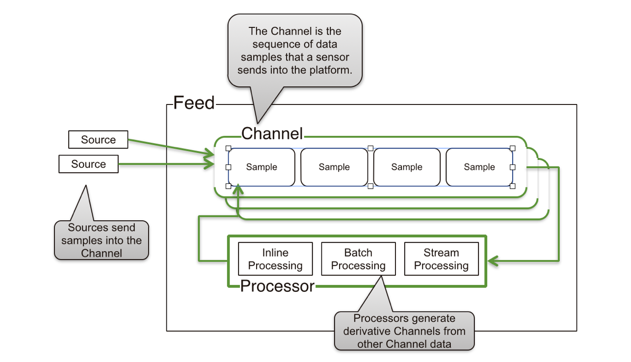
HVDF allows us to easily use MongoDB in an append-only fashion, meaning that our documents will be stored sequentially, minimizing any wasted space when we write to disk. As well, HVDF handles a number of configuration details that make MongoDB more efficient for this type of high-volume data storage, including time-based partitioning, and disabling of the default power of 2 sizes disk allocation strategy.

More information and the source code for HVDF are available on GitHub.

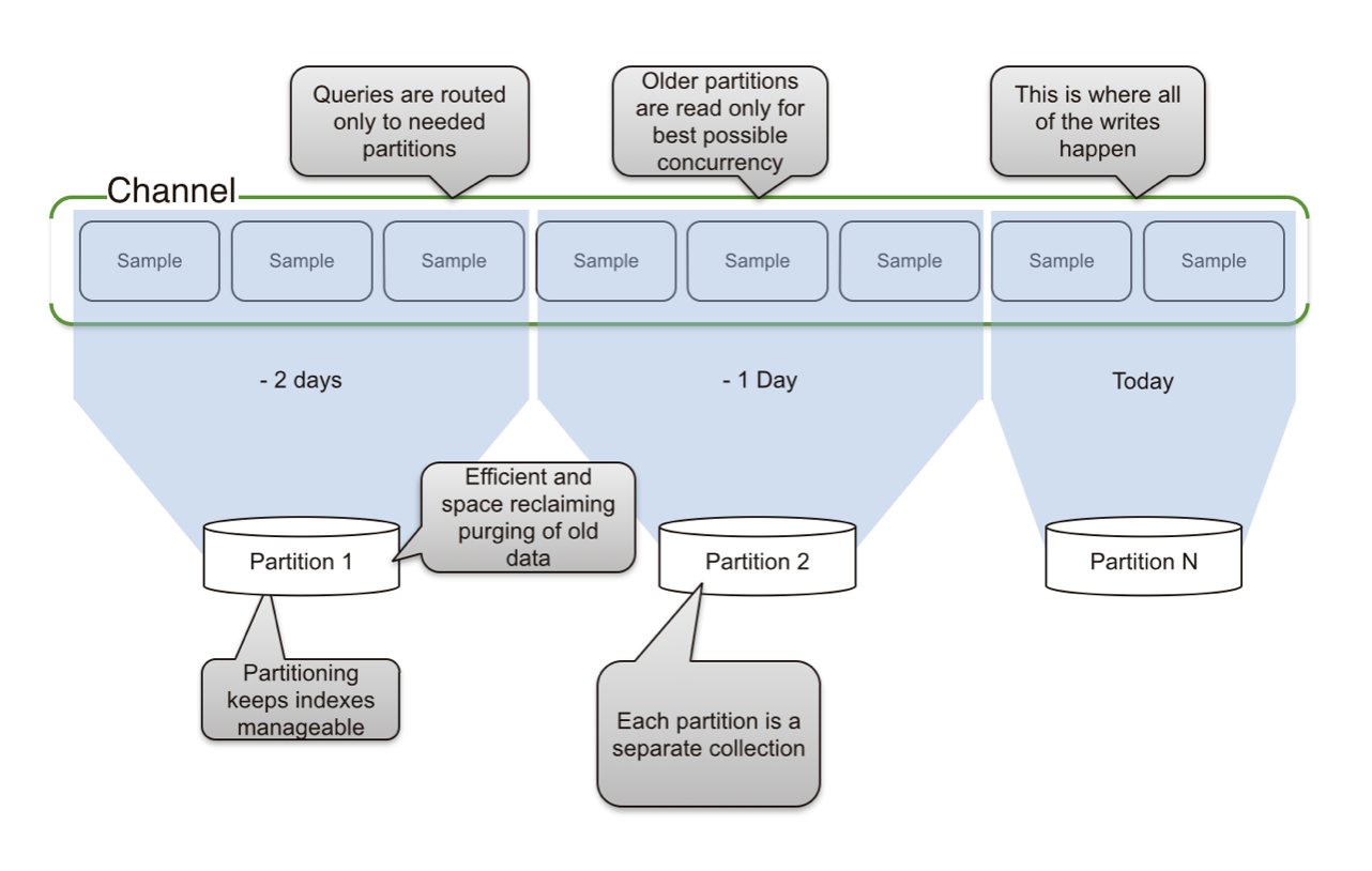
Time Partitioning

In our usage, we take advantage of HVDF’s time slicing feature, which automatically time partitions samples by creating a new collection at a specified time interval. This has four advantages:

• Sequential writes: Since a new collection is created for each time interval, samples are always written to disk sequentially.

• Fast deletes: By treating the data as sets, deletes are essentially free. All we need to do is drop the collection.

• Index size: User activity logging creates a huge amount of data. Were we to create one collection for all samples per channel our index of of those samples could quickly become huge. By slicing our channels into time intervals, we keep our indexes small enough to fit in RAM, meaning queries using those indexes remain very performant.

• Collections optimized for reads: The time interval for each collection can be configured to match the interval we are most likely to want to retrieve. In general, a best practice is to keep time partitions small enough that their indexes will fit in RAM, but large enough that you will only need to query across two collections for any given query.

• Automatic sharding: HVDF automatically creates a shard key for each time interval as the collection is created. This ensures any lookups for a given time interval are performant, since samples for the same interval are written to the same shard.

  

To specify how our data will be time partitioned, we simply pass the following to our channel configuration:

{
    "time_slicing" : 
    {
        "type"   : "periodic",
        "config" : { "period" : {"weeks" : 4} }
    }
}

In this example, we are configuring HVDF to create a new collection per channel every 4 weeks. The ‘period’ may be specified in years, weeks, hours, minutes, seconds, milliseconds or any combination of these.

Setting _id

To keep our queries highly performant, we also need to put some thought into the construction of the ‘_id’ for our documents. Since we know this data is going to be used primarily for performing time-bounded user analytics, it’s logical to choose an ‘_id’ that embeds both the creation timestamp and the ‘userID’. HVDF makes this very simple. All we need to do is specify that HVDF should use the the ‘source_time_document’ id_type channel plugin in the channel configuration:

"storage" :
{
    "type"   : "raw",
    "config" : 
    {
        "id_factory" : 
        {
            "type"   : "source_time_document",
            "config" : {  }
        }       
    }
}   
```
<p>This will give us an ‘_id’ that looks like this:</p>
<pre><code>"_id" : {
    "source" : "user457",
    "ts" : NumberLong(324000000)
}
</code></pre>

<p>By using this format for &#x2018;_id&#x2019;, we guarantee near instantaneous queries for many of the most common queries we will need in order to perform analytics on our data.</p>
<h2 id="user-insights">User Insights</h2>
<p>Now that we&#x2019;ve figured out how our user&#x2019;s activities will be logged in MongoDB, it&#x2019;s time to actually look at what we can do with that data. The first important thing to keep in mind is that, as mentioned earlier, we are trying to drink from the fire hose. Capturing this type of user data very often leads to huge data sets, so all of our queries must be time bound. Not only does this limit the number of collections that are hit by each query thanks to our time partitioning, it also keeps the amount of data being searched sane. When dealing with terabytes of data, a full table scan isn&#x2019;t even an option.</p>
<h3 id="queries">Queries</h3>
<p>Here are a couple of simple queries we might commonly use to gain some insight into a user&#x2019;s behavior. These would require secondary indexes on &#x2018;userId&#x2019; and &#x2018;itemId&#x2019;:</p>
<ul>
<li>Recent activity for a user:</li>
</ul>
<pre><code>db.activity.find({ userId: “u123”,
           ts: {“$g”t:1301284969946, // time bound the query
                 “$lt”: 1425657300} })
            .sort({ time: -1 }).limit(100) // sort in desc order
</code></pre>

<ul>
<li>Recent activity for a product:</li>
</ul>
<pre><code>db.activity.find({ itemId: “301671", // requires a secondary index on timestamp + itemId
           ts: {“$g”t:1301284969946,
                 “$lt”: 1425657300} })
            .sort({ time: -1 }).limit(100)</code></pre>

<p>To gain even more insight into what our users are doing, we can also make use of the <a href="http://docs.mongodb.org/manual/aggregation/">aggregation framework</a> in MongoDB:</p>
<ul>
<li>Recent number of views, purchases, etc for user</li>
</ul>
<pre><code>db.activities.aggregate(([
   { $match: { userId: "u123", ts: { $gt: DATE }}}, // get a time bound set of activities for a user 
   { $group: { _id: "$type", count: { $sum: 1 }}}]) // group and sum the results by activity type
</code></pre>

<ul>
<li>Recent total sales for a user</li>
</ul>
<pre><code>db.activities.aggregate(([
  { $match: { userId:"u123", ts:{$gt:DATE}, type:"ORDER"}},
   { $group: { _id: "result", count: {$sum: "$total" }}}]) // sum the total of all orders</code></pre>

<p>-Recent number of views, purchases, etc for item</p>
<pre><code>db.activities.aggregate(([
   { $match: { itemId: "301671", ts: { $gt: DATE }}}, 
   { $group: { _id: "$type", count: { $sum: 1 }}}])</code></pre>

<p>There are, of course, many different things the results of these queries might tell us about our user&#x2019;s behaviors. For example, over time, we might see that the same user has viewed the same item multiple times, meaning we might want to suggest that item to them the next time they visit our site. Similarly, we may find that a particular item has had a surge in purchases due to a sale or ad campaign, meaning we might want to suggest it to users more frequently to further drive up sales. </p>
<p>Up-selling is a big possibility here as well. For example, let&#x2019;s say we know a user has looked at several different low-end cell phones, but that in general their total purchases are relatively high. In this case, we might suggest that they look at a higher-end device that is popular amongst users with similar stats.</p>
<h3 id="map-reduce">Map-reduce</h3>
<p>Another option for performing analytics with MongoDB is to use <a href="http://docs.mongodb.org/manual/core/map-reduce/">map-reduce</a>. This is often a good choice for very large data sets when compared with the aggregation framework for a few reasons. For example, take the following aggregation that calculates the total number of times an activity has been logged in the past hour for all unique visitors:</p>
<pre><code> db.activities.aggregate(([
   { $match: { time: { $gt: NOW-1H } }}, 
   { $group: { _id: "$userId", count: {$sum: 1} } }],
   { allowDiskUse: 1 })</code></pre>

<p>Here we have several problems:</p>
<ul>
<li><p>allowDiskUse: In MongoDB, any aggregation that involves a data set greater than 100MB will throw an error, since the aggregation framework is designed to be executed in RAM. Here, the <code>allowDiskUse</code> property mitigates this issue by forcing the aggregation to be performed on disk, which as you might imagine gets extremely slow for a very large data set.</p>
</li>
<li><p>Single shard final grouping: Calculating uniques is hard for any system, but there is a particular aspect of the aggregation framework that can make performance suffer heavily. In a sharded MongoDB instance, our aggregation would first be performed per shard. Next, the results would be recombined on the primary shard and then the aggregation would be run again to remove any duplication across shards. This can become prohibitively expensive for a very large result set, particularly if the data set is large enough to require disk to be used for the aggregation.</p>
</li>
</ul>
<p>For these reasons, while map-reduce is <a href="http://blog.mongodb.org/post/62900213496/qaing-new-code-with-mms-map-reduce-vs">not always a more performant option</a> than the aggregation framework, it is better for this particular use case. Plus, the implementation is quite simple. Here&#x2019;s the same query performed with map-reduce:</p>
<pre><code> var map = function() { emit(this.userId, 1); } // emit samples by userId with value of 1
 var reduce = function(key, values) 
                          { return Array.sum(values); } // sum the total samples per user
 db.activities.mapreduce(map, reduce, 
            { query: { time: { $gt: NOW-1H } }, // time bound the query to the last hour
              out: { replace: "lastHourUniques", sharded: true }) // persist the output to a collection</code></pre>

<p>From here we can execute queries against the resulting collection:</p>
<ul>
<li>Number activities for a user in the last hour</li>
</ul>
<pre><code>db.lastHourUniques.find({ userId: "u123" })</code></pre>

<ul>
<li>Total uniques in the last hour</li>
</ul>
<pre><code>db.lastHourUniques.count()</code></pre>

<h3 id="cross-selling">Cross-selling</h3>
<p>Now to put it all together. One of the most valuable features our analytics can enable is the ability to cross-sell products to our users. For example, let&#x2019;s say a user buys a new iPhone. There&#x2019;s a vast number of related products they might also want to buy, such as cases, screen protectors, headphones, etc. By analyzing our user activity data, we can actually figure out what related items are commonly bought together and present them to the user to drive sales of additional items. Here&#x2019;s how we do it.</p>
<p>First, we calculate the items bought by a user:</p>
<pre><code> var map = function() { emit(userId, this.itemId); } // emit samples as userId: itemId
 var reduce = function(key, values) 
                      { return values; } // Return the array of itemIds the user has bought
 db.activities.mapReduce(map, reduce, 
  { query: { type: “ORDER”, time: { $gt: NOW-24H }}, // include only activities of type order int he last day
    out: { replace: "lastDayOrders", sharded: true }) // persist the output to a collection</code></pre>

<p>This will give an output collection that contains documents that look like this:</p>
<pre><code>{ _id: "u123", items: [ 2, 3, 8 ] }</code></pre>

<p>Next, we run a second map-reduce job on the outputed &#x2018;lastDayOrders&#x2019; collection to compute the number of occurrences of each item pair:</p>
<pre><code> var map = function() { 
    for (i = 0; i < this.items.length; i++) {
        for (j = i + 1; j <= this.items.length; j++) {
            emit({a: this.items[i] ,b: this.items[j] }, 1); // emit each item pair
        }
    }
}

 var reduce = function(key, values) 
                      { return Array.sum(values); } // Sum all occurrences of each item pair

 db.lastDayOrders.mapReduce(map, reduce, 
  {out: { replace: "pairs", sharded: true }) // persist the output to a collection</code></pre>

<p>This will give us an output collection that contains a count of how many times each set of items has been ordered together. The collection will contain documents that look like this:</p>
<pre><code>{ _id: { a: 2, b: 3 }, value: 36 }</code></pre>

<p>All we need to do from here is to create a secondary index on each item and its count, e.g. <code>{_id.a:&#x201D;u123&#x201D;, count:36}</code>. This makes determining which items to cross-sell a matter of a simple query to retrieve the items most commonly ordered together. In the following example, we retrieve only those items that have been ordered with itemId u123 more than 10 times, and sort in descending order: </p>
<pre><code>db.pairs.find( { _id.a: "u123", count: { $gt: 10 }} )
             .sort({ count: -1 })</code></pre>

<p>We can also optionally make the data more compact by grouping the most popular pairs in a separate collection, like this:</p>
<pre><code>{ itemId: 2, recom: [ { itemId: 32, weight: 36}, 
                        { itemId: 158, weight: 23},
                           … ] }</code></pre>

<h2 id="hadoop-integration">Hadoop Integration</h2>
<p>For many applications, either using the aggregation framework for real-time data analytics, or the map-reduce function for less frequent handling of large data sets in MongoDB are great options, but clearly, for complex number crunching of truly massive datasets, <a href="http://hadoop.apache.org">Hadoop</a> is going to be the tool of choice. For this reason, we have created a <a href="https://github.com/mongodb/mongo-hadoop">Hadoop connector</a> for MongoDB that makes processing data from a MongoDB cluster in Hadoop a much simpler task. Here are just a few of the features:</p>
<ul>
<li>Read/write from MongoDB or exported BSON</li>
<li>Integration with Pig, Spark, Hive, MapReduce and others</li>
<li>Works with Apache Hadoop, Cloudera CDH, Hortonworks HDP</li>
<li>Open source</li>
<li>Support for filtering with MongoDB queries, authentication, reading from replica set tags, and more</li>
</ul>
<p>For more information on the MongoDB Hadoop connector, check out the project on <a href="https://github.com/mongodb/mongo-hadoop">GitHub</a>.</p>
<h2 id="recap">Recap</h2>
<p>Performing user analytics, whether in real-time or incrementally, is no small task. Every step of the process from capturing user data, to data storage, to data retrieval, to crunching the numbers present challenges that require significant planning if the system is to perform well. Luckily, MongoDB and HVDF can be great tools for accomplishing these types of tasks, either on their own or used in conjunction with other tools like Hadoop.</p>
<p>That&#x2019;s it for our four part series on retail reference architecture! In just four blog posts we&#x2019;ve covered how MongoDB can be used to power some of the most common and complex needs of large-scale retailers, including <a href="https://www.mongodb.com/blog/post/retail-reference-architecture-part-1-building-flexible-searchable-low-latency-product">product catalogs</a>, <a href="https://www.mongodb.com/blog/post/retail-reference-architecture-part-2-approaches-inventory-optimization">inventory</a>, and <a href="https://www.mongodb.com/blog/post/retail-reference-architecture-part-3-query-optimization-and-scaling">query optimization</a>. For more tools and examples of what MongoDB can do for you, check out our <a href="https://github.com/mongodb/">GitHub</a>.</p>
<h2 id="learn-more">Learn more</h2>
<p>To discover how you can re-imagine the retail experience with MongoDB, <a href="https://www.mongodb.com/lp/white-paper/serving-the-digitally-oriented-consumer?jmp=blog" target="_blank">read our white paper</a>. In this paper, you&apos;ll learn about the new retail challenges and how MongoDB addresses them.</p>
<p></p><hr>
Learn more about how leading brands differentiate themselves with technologies and processes that enable the omni-channel retail experience.<p></p>
<p></p><center><a class="btn btn-primary" href="https://www.mongodb.com/collateral/serving-digitally-oriented-consumer?jmp=blog" target="_BLANK">Read our guide on the digitally oriented consumer</a></center><p></p>
<hr>

<p style="float:left; margin-bottom:0px;font-size: 18px;"><strong><a href="https://www.mongodb.com/blog/post/retail-reference-architecture-part-3-query-optimi

 

 

转载于 《https://www.mongodb.com/blog/post/retail-reference-architecture-part-4-recommendations-and-personalizations》