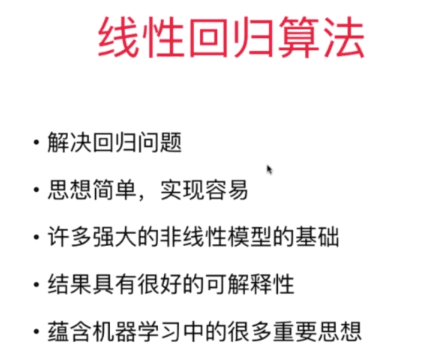
简单的线性回归算法
一.认识回归
1.简单的介绍
回归是统计学中最有力的工具之一。机器学习监督学习算法分为分类算法和回归算法两种,其实就是根据类别标签分布类型为离散型、连续性而定义的。顾名思义,分类算法用于离散型分布预测,如决策树、朴素贝叶斯、adaboost、SVM、Logistic回归都是分类算法;回归算法用于连续型分布预测,针对的是数值型的样本,使用回归,可以在给定输入的时候预测出一个数值,这是对分类方法的提升,因为这样可以预测连续型数据而不仅仅是离散的类别标签。
回归的目的就是建立一个回归方程用来预测目标值,回归的求解就是求这个回归方程的回归系数。预测的方法当然十分简单,回归系数乘以输入值再全部相加就得到了预测值。
2.回归的定义
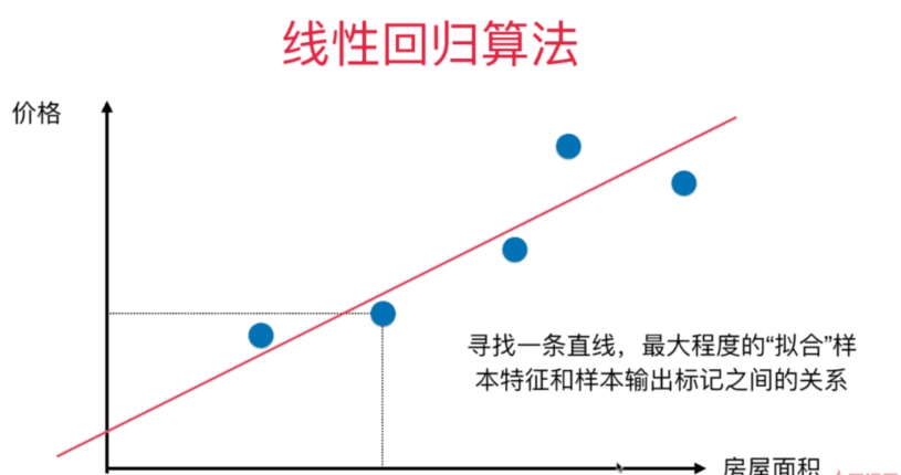
回归最简单的定义是,给出一个点集D,用一个函数去拟合这个点集,并且使得点集与拟合函数间的误差最小,如果这个函数曲线是一条直线,那就被称为线性回归,如果曲线是一条二次曲线,就被称为二次回归。
3.多元线性回归
在回归分析中,如果有两个或两个以上的自变量,就称为多元回归。事实上,一种现象常常是与多个因素相联系的,由多个自变量的最优组合共同来预测或估计因变量,比只用一个自变量进行预测或估计更有效,更符合实际。因此多元线性回归比一元线性回归的实用意义更大。
特别注意:注意多元和多次是两个不同的概念,“多元”指方程有多个参数,“多次”指的是方程中参数的最高次幂。多元线性方程是假设预测值y与样本所有特征值符合一个多元一次线性方程。
二.线性回归算法
1.简单介绍
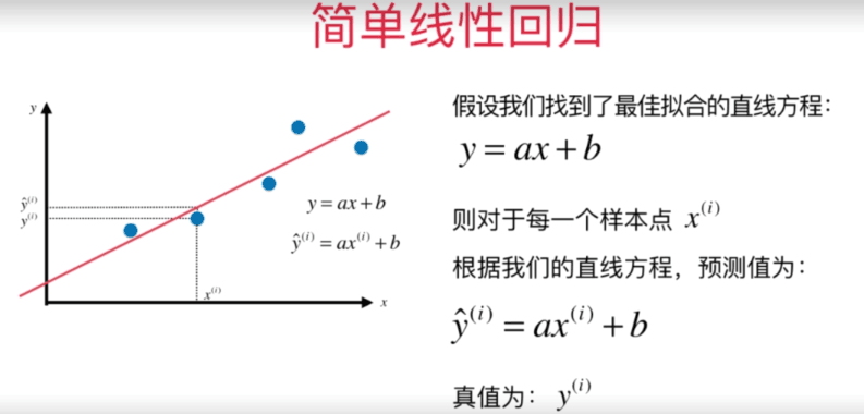
由上图可知,我们必须要求出y=ax + b的最佳拟合直线,因此我们需要先求出参数a和参数b的值,这里我们采用最小二乘法的方法进行求解
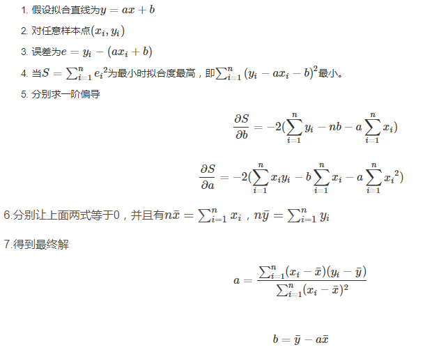
2.线性回归的求解方法--最小二乘法
线性回归过程主要解决的就是如何通过样本来获取最佳的拟合线。最常用的方法便是最小二乘法,它是一种数学优化技术,它通过最小化误差的平方和寻找数据的最佳函数匹配。
1.数学公式推导
示例代码:
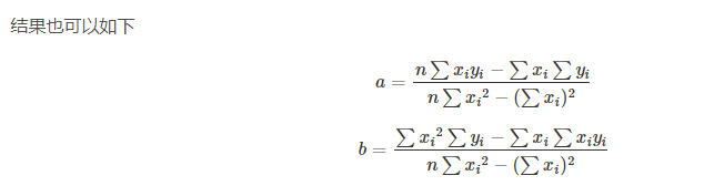
import numpy as np
import matplotlib.pyplot as plt

#自己创建几个虚拟的数据
x = np.array([1.,2.,3.,4.,5.])
y = np.array([1.,3.,2.,3.,5.])

#绘制出大致的散点图片
plt.scatter(x,y)
plt.axis([0,6,0,6])
plt.show()     #图1


#求出相应的平均值
x_mean=np.mean(x)
y_mean=np.mean(y)


#根据推导公式求出参数a 和 参数b的值
num = 0.0
d = 0.0
for x_i,y_i in zip(x,y):
    num += (x_i - x_mean) * (y_i - y_mean)
    d += (x_i - x_mean) ** 2

a = num / d
b = y_mean - a * x_mean

y_hat = a * x + b

#可视化数据的处理
plt.scatter(x,y)
plt.plot(x,y_hat,color = 'red')
plt.axis([0,6,0,6])
plt.show()  #图2
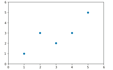
图1
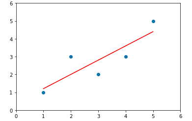
图2
根据求出的a和b进行预测
x_predict=6
y_predict= a * x_predict + b

y_predict   #5.2
2.封装代码并实现
import numpy as np

class SimpleLinearRegression():

    def __init__(self):
        """初始化Simple Linear Regression模型"""
        self.a_=None
        self.b_=None

    def fit(self,x_train,y_train):

        """根据训练数据集x_train, y_train训练Simple Linear Regression模型"""
        assert x_train.ndim == 1, \
            "Simple Linear Regressor can only solve single feature training data."
        assert len(x_train) == len(y_train), \
            "the size of x_train must be equal to the size of y_train"
        x_mean = np.mean(x_train)
        y_mean = np.mean(y_train)

        num = 0.0
        d = 0.0
        for x_i, y_i in zip(x_train, y_train):
            num += (x_i - x_mean) * (y_i - y_mean)
            d += (x_i - x_mean) ** 2

        self.a_= num / d
        self.b_=y_mean - self.a_ * x_mean

        return self

    def predict(self,x_predict):
        """给定待预测数据集x_predict,返回表示x_predict的结果向量"""
        assert x_predict.ndim == 1, \
            "Simple Linear Regressor can only solve single feature training data."
        assert self.a_ is not None and self.b_ is not None, \
            "must fit before predict!"

        return np.array([self._predict(x) for x in x_predict])

    def _predict(self,x_train):
        """给定单个待预测数据x,返回x的预测结果值"""
        return self.a_ * x_train + self.b_

    def __repr__(self):
        return "SimpleLinearRegression()"
在jupyter notebook上进行相关的测试
%run D:\project\sk-learn\Linear_regression\simple_linear_regression.py

#先实例化一个对象
simplelinearregression=SimpleLinearRegression()

#让对象调用fit方法
simplelinearregression.fit(x,y)  #


simplelinearregression.a_  #参数a的值:0.8

simplelinearregression.b_ #参数b的值:0.39999999999999947

y_hat= simplelinearregression.a_ * x + simplelinearregression.b_


#数据可是化处理
plt.scatter(x,y)
plt.plot(x,y_hat,color = 'red')
plt.axis([0,6,0,6])
plt.show()
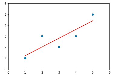
图3
可以上图和前面的可视化结果是基本上是一样的,因此该实现方式的方法是可行的
3.采用向量的计算方法来进行计算
上面的代码是实现了计算线性回归的方法,但是该代码的执行时间花费较长,因此我们采用向量的计算方法来进行相应的优化
示例代码如下:
import numpy as np

class SimpleLinearRegression2():

    def __init__(self):
        """初始化Simple Linear Regression模型"""
        self.a_=None
        self.b_=None

    def fit(self,x_train,y_train):

        """根据训练数据集x_train, y_train训练Simple Linear Regression模型"""
        assert x_train.ndim == 1, \
            "Simple Linear Regressor can only solve single feature training data."
        assert len(x_train) == len(y_train), \
            "the size of x_train must be equal to the size of y_train"
        x_mean = np.mean(x_train)
        y_mean = np.mean(y_train)

        self.a_= (x_train - x_mean).dot(y_train - y_mean) / (x_train - x_mean).dot(x_train - x_mean)
        self.b_=y_mean - self.a_ * x_mean

        return self

    def predict(self,x_predict):
        """给定待预测数据集x_predict,返回表示x_predict的结果向量"""
        assert x_predict.ndim == 1, \
            "Simple Linear Regressor can only solve single feature training data."
        assert self.a_ is not None and self.b_ is not None, \
            "must fit before predict!"

        return np.array([self._predict(x) for x in x_predict])

    def _predict(self,x_train):
        """给定单个待预测数据x,返回x的预测结果值"""
        return self.a_ * x_train + self.b_

    def __repr__(self):
        return "SimpleLinearRegression2()"
在jupyter notebook上进行相关的测试
%run D:\project\sk-learn\Linear_regression\simple_linear_regression.py

#先实例化一个对象
simplelinearregression=SimpleLinearRegression2()

#让对象调用fit方法
simplelinearregression2.fit(x,y)  #


simplelinearregression2.a_  #参数a的值:0.8

simplelinearregression2.b_ #参数b的值:0.39999999999999947

y_hat2= simplelinearregression2.a_ * x + simplelinearregression2.b_


#数据可是化处理
plt.scatter(x,y)
plt.plot(x,y_hat2,color = 'red')
plt.axis([0,6,0,6])
plt.show()
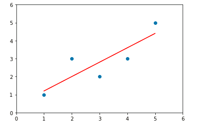
图4
由图可知图4和图3的结果是一样的
4.测试两种计算方法运行速度
1.在jupyter notebook上进行测试
m = 1000000
big_x = np.random.random(size=m)  #创建一个随机的数组
big_y = big_x * 2.0 + 3.0 + np.random.normal(size=m) #最后这个是加上一点误差


#测试两种算法的运行时间
%timeit simplelinearregression.fit(big_x,big_y)
%timeit simplelinearregression2.fit(big_x,big_y)

#2.42 s ± 151 ms per loop (mean ± std. dev. of 7 runs, 1 loop each)
#21.9 ms ± 271 µs per loop (mean ± std. dev. of 7 runs, 10 loops each)

#由上述结果可以知道,向量的方法比普通的方法快了100倍左右

 浙公网安备 33010602011771号