
python实现多分类评价指标
1、什么是多分类?
参考:https://www.jianshu.com/p/9332fcfbd197
针对多类问题的分类中,具体讲有两种,即multiclass classification和multilabel classification。multiclass是指分类任务中包含不止一个类别时,每条数据仅仅对应其中一个类别,不会对应多个类别。multilabel是指分类任务中不止一个分类时,每条数据可能对应不止一个类别标签,例如一条新闻,可以被划分到多个板块。
无论是multiclass,还是multilabel,做分类时都有两种策略,一个是one-vs-the-rest(one-vs-all),一个是one-vs-one。
在one-vs-all策略中,假设有n个类别,那么就会建立n个二项分类器,每个分类器针对其中一个类别和剩余类别进行分类。进行预测时,利用这n个二项分类器进行分类,得到数据属于当前类的概率,选择其中概率最大的一个类别作为最终的预测结果。
在one-vs-one策略中,同样假设有n个类别,则会针对两两类别建立二项分类器,得到k=n*(n-1)/2个分类器。对新数据进行分类时,依次使用这k个分类器进行分类,每次分类相当于一次投票,分类结果是哪个就相当于对哪个类投了一票。在使用全部k个分类器进行分类后,相当于进行了k次投票,选择得票最多的那个类作为最终分类结果。
2、构建多个二分类器进行分类
使用的数据集是sklearn自带的iris数据集,该数据集总共有三类。
import numpy as np
import matplotlib.pyplot as plt
from sklearn import svm,datasets
from itertools import cycle

from sklearn import svm, datasets
from sklearn.metrics import roc_curve, auc
from sklearn.model_selection import train_test_split
from sklearn.preprocessing import label_binarize
from sklearn.multiclass import OneVsRestClassifier
from scipy import interp

# 导入鸢尾花数据集
iris = datasets.load_iris()
X = iris.data  # X.shape==(150, 4)
y = iris.target  # y.shape==(150, )

# 二进制化输出
y = label_binarize(y, classes=[0, 1, 2])  # shape==(150, 3)
n_classes = y.shape[1]  # n_classes==3

#np.r_是按列连接两个矩阵,就是把两矩阵上下相加,要求列数相等。
#np.c_是按行连接两个矩阵,就是把两矩阵左右相加,要求行数相等。
# 添加噪音特征,使问题更困难
random_state = np.random.RandomState(0)
n_samples, n_features = X.shape  # n_samples==150, n_features==4
X = np.c_[X, random_state.randn(n_samples, 200 * n_features)]  # shape==(150, 84)
# 打乱数据集并切分训练集和测试集
X_train, X_test, y_train, y_test = train_test_split(X, y, test_size=.5,
                                                    random_state=0)
# X_train.shape==(75, 804), X_test.shape==(75, 804), y_train.shape==(75, 3), y_test.shape==(75, 3)

# 学习区分某个类与其他的类
classifier = OneVsRestClassifier(svm.SVC(kernel='linear', probability=True,
                                 random_state=random_state))
y_score = classifier.fit(X_train, y_train).decision_function(X_test)
这里提一下classifier.fit()后面接的函数:可以是decision_function()、predict_proba()、predict()
predict():返回预测标签、
predict_proba():返回预测属于某标签的概率
decision_function():返回样本到分隔超平面的有符号距离来度量预测结果的置信度
这里我们分别打印一下对应的y_score,只取前三条数据:
预测标签:[[0 0 1] [0 1 0] [1 0 0]...]
概率:[[6.96010030e-03 1.67062907e-01 9.65745632e-01] [4.57532814e-02 3.05231268e-01 4.58939259e-01] [7.00832624e-01 2.32537226e-01 4.92996070e-02]...]
距离:[[-1.18047012 -2.60334173 1.48134717] [-0.72354789 0.15798952 -0.08648247] [ 0.22439326 -1.15044791 -1.35488445]...]
同时,我们还要注意使用到了:OneVsRestClassifier,如何理解呢?
我们可以这么看:OneVsRestClassifier实际上包含了多个分类器,有多少个类别就有多少个分类器,这里有三个类别,因此就有三个分类器,可以通过:
print(classifier.estimators_)
来查看:
[SVC(C=1.0, break_ties=False, cache_size=200, class_weight=None, coef0=0.0,
    decision_function_shape='ovr', degree=3, gamma='scale', kernel='linear',
    max_iter=-1, probability=True,
    random_state=RandomState(MT19937) at 0x7F480F316A98, shrinking=True,
    tol=0.001, verbose=False),
SVC(C=1.0, break_ties=False, cache_size=200, class_weight=None, coef0=0.0,
    decision_function_shape='ovr', degree=3, gamma='scale', kernel='linear',
    max_iter=-1, probability=True,
    random_state=RandomState(MT19937) at 0x7F480F316CA8, shrinking=True,
    tol=0.001, verbose=False),
SVC(C=1.0, break_ties=False, cache_size=200, class_weight=None, coef0=0.0,
    decision_function_shape='ovr', degree=3, gamma='scale', kernel='linear',
    max_iter=-1, probability=True,
    random_state=RandomState(MT19937) at 0x7F480F316DB0, shrinking=True,
    tol=0.001, verbose=False)]
对于每一个分类器,都是二分类,即将当前的类视为一类,另外的其他类视为一类,比如说我们可以取得其中的分类器进行分类,以第一个标签为例:
y_true=np.where(y_test==1)[1]
array([2, 1, 0, 2, 0, 2, 0, 1, 1, 1, 2, 1, 1, 1, 1, 0, 1, 1, 0, 0, 2, 1, 0, 0, 2, 0, 0, 1, 1, 0, 2, 1, 0, 2, 2, 1, 0, 1, 1, 1, 2, 0, 2, 0, 0, 1, 2, 2, 2, 2, 1, 2, 1, 1, 2, 2, 2, 2, 1, 2, 1, 0, 2, 1, 1, 1, 1, 2, 0, 0, 2, 1, 0, 0, 1])
#这里重新定义标签,1代表当前标签,0代表其他标签
y0=[0 if i==0 else 1 for i in y_true]
print(y0)
print(classifier.estimators_[0].fit(X_train,y0).predict(X_test))
[0, 0, 1, 0, 1, 0, 1, 0, 0, 0, 0, 0, 0, 0, 0, 1, 0, 0, 1, 1, 0, 0, 1, 1, 0, 1, 1, 0, 0, 1, 0, 0, 1, 0, 0, 0, 1, 0, 0, 0, 0, 1, 0, 1, 1, 0, 0, 0, 0, 0, 0, 0, 0, 0, 0, 0, 0, 0, 0, 0, 0, 1, 0, 0, 0, 0, 0, 0, 1, 1, 0, 0, 1, 1, 0]
[0 0 1 1 1 0 0 0 0 0 0 0 0 0 0 0 0 0 0 0 0 1 0 0 1 0 0 0 0 0 1 0 1 0 0 0 0 0 0 0 1 1 0 1 1 1 1 0 0 0 0 0 0 1 0 1 0 1 0 1 0 0 0 1 0 1 0 1 0 0 1 0 1 0 0]
我们直接打印y_score中第0列的结果y_score[:,0]:
[0 0 1 0 1 0 1 0 0 0 0 0 0 0 0 1 0 0 1 1 0 0 1 1 0 1 1 0 0 1 0 0 1 0 0 0 1 0 0 0 0 1 0 1 1 0 0 0 0 0 0 0 0 0 0 0 0 0 0 0 0 1 0 0 0 0 0 0 1 1 0 0 1 1 0]
就是对应的第一个分类器的结果。(这里的结果不一致是因为classifier.estimators_[0].fit(X_train,y0).predict(X_test)相当于有重新训练并预测了一次。
从而,y_score中的每一列都表示了每一个分类器的结果。
所以,在y_score的结果中出现了:[1,1,0]这种就不足为怪了。但是有个问题,如果其中有两个分类器都将某个类认为是当前类,那么这类到底属于哪一个类呢?所以不能直接就对每一个分类器的概率值取得标签值,而是要计算出每一个分类器的概率值,最后再进行映射成标签。回过头来才发现的,以下使用的是predict(),因此是有问题的,但是基本方式是差不多的,再修改就有点麻烦了,酌情阅读了= =。
多分类问题就转换为了oneVsRest问题,可以分别使用二分类评价指标了,可参考:
https://www.cnblogs.com/xiximayou/p/13682052.html
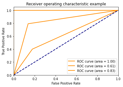
比如说绘制ROC和计算AUC:
from sklearn.metrics import roc_curve, auc
# 为每个类别计算ROC曲线和AUC
fpr = dict()
tpr = dict()
roc_auc = dict()
n_classes=3
for i in range(n_classes):
    fpr[i], tpr[i], _ = roc_curve(y_test[:, i], y_score[:, i])
    roc_auc[i] = auc(fpr[i], tpr[i])
# fpr[0].shape==tpr[0].shape==(21, ), fpr[1].shape==tpr[1].shape==(35, ), fpr[2].shape==tpr[2].shape==(33, )
# roc_auc {0: 0.9118165784832452, 1: 0.6029629629629629, 2: 0.7859477124183007}

plt.figure()
lw = 2
for i in range(n_classes):
  plt.plot(fpr[i], tpr[i], color='darkorange',
          lw=lw, label='ROC curve (area = %0.2f)' % roc_auc[i])
plt.plot([0, 1], [0, 1], color='navy', lw=lw, linestyle='--')
plt.xlim([0.0, 1.0])
plt.ylim([0.0, 1.05])
plt.xlabel('False Positive Rate')
plt.ylabel('True Positive Rate')
plt.title('Receiver operating characteristic example')
plt.legend(loc="lower right")
plt.show()
3、多分类评价指标?
宏平均 Macro-average
Macro F1:将n分类的评价拆成n个二分类的评价,计算每个二分类的F1 score,n个F1 score的平均值即为Macro F1。
微平均 Micro-average
Micro F1:将n分类的评价拆成n个二分类的评价,将n个二分类评价的TP、FP、TN、FN对应相加,计算评价准确率和召回率,由这2个准确率和召回率计算的F1 score即为Micro F1。
对于二分类问题:
TP=cnf_matrix[1][1] #预测为正的真实标签为正
FP=cnf_matrix[0][1] #预测为正的真实标签为负
FN=cnf_matrix[1][0] #预测为负的真实标签为正
TN=cnf_matrix[0][0] #预测为负的真实标签为负
accuracy=(TP+TN)/(TP+FP+FN+TN)
precision=TP/(TP+FP)
recall=TP/(TP+FN)
f1score=2 * precision * recall/(precision + recall)
ROC曲线:
横坐标:假正率(False positive rate, FPR),预测为正但实际为负的样本占所有负例样本的比例;
FPR = FP / ( FP +TN)
纵坐标:真正率(True positive rate, TPR),这个其实就是召回率,预测为正且实际为正的样本占所有正例样本的比例。
TPR = TP / ( TP+ FN)
AUC:就是roc曲线和横坐标围城的面积。
对于上述的oneVsRest:
# 计算微平均ROC曲线和AUC
fpr["micro"], tpr["micro"], _ = roc_curve(y_test.ravel(), y_score.ravel())
roc_auc["micro"] = auc(fpr["micro"], tpr["micro"])

# 计算宏平均ROC曲线和AUC

# 首先汇总所有FPR
all_fpr = np.unique(np.concatenate([fpr[i] for i in range(n_classes)]))

# 然后再用这些点对ROC曲线进行插值
mean_tpr = np.zeros_like(all_fpr)
for i in range(n_classes):
    mean_tpr += interp(all_fpr, fpr[i], tpr[i])

# 最后求平均并计算AUC
mean_tpr /= n_classes

fpr["macro"] = all_fpr
tpr["macro"] = mean_tpr
roc_auc["macro"] = auc(fpr["macro"], tpr["macro"])

# 绘制所有ROC曲线
plt.figure()
lw = 2
plt.plot(fpr["micro"], tpr["micro"],
         label='micro-average ROC curve (area = {0:0.2f})'
               ''.format(roc_auc["micro"]),
         color='deeppink', linestyle=':', linewidth=4)

plt.plot(fpr["macro"], tpr["macro"],
         label='macro-average ROC curve (area = {0:0.2f})'
               ''.format(roc_auc["macro"]),
         color='navy', linestyle=':', linewidth=4)

colors = cycle(['aqua', 'darkorange', 'cornflowerblue'])
for i, color in zip(range(n_classes), colors):
    plt.plot(fpr[i], tpr[i], color=color, lw=lw,
             label='ROC curve of class {0} (area = {1:0.2f})'
             ''.format(i, roc_auc[i]))

plt.plot([0, 1], [0, 1], 'k--', lw=lw)
plt.xlim([0.0, 1.0])
plt.ylim([0.0, 1.05])
plt.xlabel('False Positive Rate')
plt.ylabel('True Positive Rate')
plt.title('Some extension of Receiver operating characteristic to multi-class')
plt.legend(loc="lower right")
plt.show()

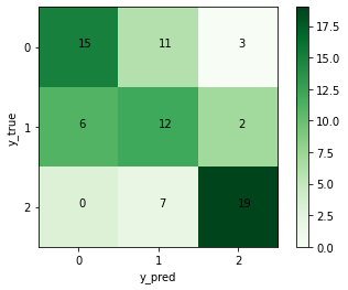
接下来我们将分类视为一个整体:
from sklearn.metrics import confusion_matrix
classes=[0,1,2]
y_my_test=np.where(y_test==1)[1]
y_my_score=np.zeros(y_my_test.shape)
for i in range(len(classes)):
  y_my_score[np.where(y_score[:,i]==1)]=i
confusion = confusion_matrix(y_my_test, y_my_score)# 绘制热度图
plt.imshow(confusion, cmap=plt.cm.Greens)
indices = range(len(confusion))
plt.xticks(indices, classes)
plt.yticks(indices, classes)
plt.colorbar()
plt.xlabel('y_pred')
plt.ylabel('y_true')

# 显示数据
for first_index in range(len(confusion)):
  for second_index in range(len(confusion[first_index])):
    plt.text(first_index, second_index, confusion[first_index][second_index])

# 显示图片
plt.show()
我们首先要将测试标签和预测标签转换为非One-hot编码,才能计算出混淆矩阵:
计算出每一类的评价指标:
from sklearn.metrics import classification_report
t = classification_report(y_my_test, y_my_score, target_names=['0', '1', '2'])
              precision    recall  f1-score   support

           0       0.52      0.71      0.60        21
           1       0.60      0.40      0.48        30
           2       0.73      0.79      0.76        24

    accuracy                           0.61        75
   macro avg       0.62      0.64      0.61        75
weighted avg       0.62      0.61      0.60        75
如果要使用上述的值,需要这么使用:
t = classification_report(y_my_test, y_my_score, target_names=['0', '1', '2'],output_dict=True)
{'0': {'precision': 0.5172413793103449, 'recall': 0.7142857142857143, 'f1-score': 0.6000000000000001, 'support': 21}, '1': {'precision': 0.6, 'recall': 0.4, 'f1-score': 0.48, 'support': 30}, '2': {'precision': 0.7307692307692307, 'recall': 0.7916666666666666, 'f1-score': 0.76, 'support': 24}, 'accuracy': 0.6133333333333333, 'macro avg': {'precision': 0.6160035366931919, 'recall': 0.6353174603174603, 'f1-score': 0.6133333333333334, 'support': 75}, 'weighted avg': {'precision': 0.6186737400530504, 'recall': 0.6133333333333333, 'f1-score': 0.6032000000000001, 'support': 75}}
我们可以分别计算每一类的相关指标:
import sklearn
for i in range(len(classes)):
  precision=sklearn.metrics.precision_score(y_test[:,i], y_score[:,i], labels=None, pos_label=1, average='binary',
                                sample_weight=None)
  print("{} precision:{}".format(i,precision))
也可以整体计算:
from sklearn.metrics import precision_score
print(precision_score(y_test, y_score, average="micro"))
average可选参数micro、macro、weighted
具体的计算方式可以去参考:
https://zhuanlan.zhihu.com/p/59862986
参考:
https://blog.csdn.net/hfutdog/article/details/88079934

 浙公网安备 33010602011771号