


决策树模型系列——10、XGBoost使用案例
from sklearn.datasets import fetch_california_housing, load_digits
from sklearn.metrics import confusion_matrix, mean_squared_error, accuracy_score
from sklearn.model_selection import  train_test_split
import xgboost as xgb
import matplotlib.pyplot as plt
from hyperopt import hp, fmin, tpe, Trials
1、XGBoost原生接口
官方文档:Python API Reference — xgboost 2.0.3 documentation
二分类
X, y = load_digits(n_class=2, return_X_y=True)

X_train, X_test, y_train, y_test = train_test_split(X, y, test_size=0.2)
# 训练集和测试集数据
dtrain = xgb.DMatrix(X_train, y_train)
dtest = xgb.DMatrix(X_test, y_test)

# 模型参数设置
params = {
    "max_depth": 2,
    "objective": "binary:logistic",
    "eval_metric": ["error"],
}
num_booster_round = 50

# 模型训练
dst = xgb.train(
    params, dtrain,
    num_booster_round,
    evals=[(dtrain, 'train'), (dtest, 'test')], # 验证数据集
    early_stopping_rounds = 5
)

# 预测结果
preds = bst.predict(dtest)

# 预测准确度
print('--'*25)
print(f"预测准确度:{accuracy_score(y_test, preds):.3f}")

# 混淆矩阵
print('--'*25)
print("混淆矩阵:")
print(confusion_matrix(y_test, preds))
[0]	train-error:0.00347	test-error:0.00000
[1]	train-error:0.00347	test-error:0.00000
[2]	train-error:0.00000	test-error:0.01389
[3]	train-error:0.00000	test-error:0.01389
[4]	train-error:0.00000	test-error:0.00000
--------------------------------------------------
预测准确度:1.000
--------------------------------------------------
混淆矩阵:
[[36  0]
 [ 0 36]]
多分类
X, y = load_digits(n_class=10, return_X_y=True)

X_train, X_test, y_train, y_test = train_test_split(X, y, test_size=0.2)
# 训练数据和测试数据
dtrain = xgb.DMatrix(X_train, y_train)
dtest = xgb.DMatrix(X_test, y_test)

# 模型参数设置
params = {
    "booster": "gbtree",
    "verbosity": 1,
    "eta": 0.8,
    "gamma":0,
    "max_depth": 2,
    "subsample": 1,
    "colsample_bytree": 1,
    "colsample_bylevel": 1,
    "colsample_bynode": 1,
    "lambda": 1,
    "alpha": 0,
    "tree_method": "hist",
    "max_bin": 256,
    "objective": "multi:softmax",
    "eval_metric": ["merror"],
    "num_class": 10      #多分类时需要设置num_class = 标签类别个数
}
num_booster_round = 200

# 模型训练
print("训练过程...")
bst = xgb.train(
        params,
        dtrain,
        num_booster_round,
        evals=[(dtrain, 'train'),(dtest, 'test')],  # early_stopping_rounds的验证集
        early_stopping_rounds = 10
    )

# 预测结果(测试集)
preds = bst.predict(dtest, iteration_range=(0, bst.best_iteration + 1))

# 预测准确度
print('--'*25)
print(f"预测准确度:{accuracy_score(y_test, preds):.3f}")

# 混淆矩阵
print('--'*25)
print("混淆矩阵:")
print(confusion_matrix(y_test, preds))
训练过程...
[0]	train-merror:0.19068	test-merror:0.26111
[1]	train-merror:0.14475	test-merror:0.19167
[2]	train-merror:0.09673	test-merror:0.16389
[3]	train-merror:0.07168	test-merror:0.13333
[4]	train-merror:0.04593	test-merror:0.11667
[5]	train-merror:0.03271	test-merror:0.10000
[6]	train-merror:0.01740	test-merror:0.08611
[7]	train-merror:0.01322	test-merror:0.07500
[8]	train-merror:0.01044	test-merror:0.07222
[9]	train-merror:0.00696	test-merror:0.06944
[10]	train-merror:0.00348	test-merror:0.05833
[11]	train-merror:0.00278	test-merror:0.05833
[12]	train-merror:0.00139	test-merror:0.05556
[13]	train-merror:0.00070	test-merror:0.06111
[14]	train-merror:0.00070	test-merror:0.05833
[15]	train-merror:0.00070	test-merror:0.05833
[16]	train-merror:0.00000	test-merror:0.06111
[17]	train-merror:0.00070	test-merror:0.06111
[18]	train-merror:0.00000	test-merror:0.05833
[19]	train-merror:0.00000	test-merror:0.06111
[20]	train-merror:0.00000	test-merror:0.05833
[21]	train-merror:0.00000	test-merror:0.05833
[22]	train-merror:0.00000	test-merror:0.05833
--------------------------------------------------
预测准确度:0.944
--------------------------------------------------
混淆矩阵:
[[37  0  0  0  0  0  0  0  0  0]
 [ 0 33  1  1  0  0  0  0  0  2]
 [ 1  1 34  2  0  0  0  0  0  1]
 [ 0  0  0 30  0  0  0  1  0  0]
 [ 0  1  0  0 36  0  0  0  0  0]
 [ 0  0  0  0  0 35  0  0  1  2]
 [ 0  0  0  0  0  0 45  0  0  0]
 [ 0  0  0  1  0  0  0 33  0  1]
 [ 0  2  0  1  0  0  0  1 31  0]
 [ 0  0  0  0  0  0  0  0  0 26]]
回归
# 导入数据集,并拆分为训练集和测试集
X, y = fetch_california_housing(return_X_y=True)
X_train, X_test, y_train, y_test = train_test_split(X, y, test_size=0.2, shuffle=True)
# 构造训练集和测试集
dtrain = xgb.DMatrix(X_train, y_train)
dtest = xgb.DMatrix(X_test, y_test)

# 参数设置(使用hyperopt搜索)
space = {
    "eta": hp.uniform("eta", 0.01, 0.1),
    "gamma": hp.choice("gamma", [0, 1, 2, 3]),
    "max_depth": hp.choice("max_depth", [1, 6, 12]),
}
num_boost_round = 1000

# 目标函数
def objective(params):
    bst = xgb.train(
        params,dtrain,
        num_boost_round=num_boost_round,
        evals=[(dtrain, 'train'), (dtest, 'test')], # 验证数据集
        early_stopping_rounds = 5
    )
    preds = bst.predict(dtest)
    mse = mean_squared_error(y_test, preds)
    return mse


# 运行Hyperopt
trials = Trials()
best = fmin(fn=objective,
            space=space,
            algo=tpe.suggest,
            max_evals=50,
            trials=trials
           )
print(f"Best-Hyper: {best}")
100%|███████████████████████████████████████████████| 50/50 [22:22<00:00, 26.84s/trial, best loss: 0.22942034509119466]
Best-Hyper: {'eta': 0.08393671868894494, 'gamma': 0, 'max_depth': 1}
cv_result = xgb.cv(best, dtrain, num_boost_round=1000)

# bst = xgb.train(
#     best,dtrain,
#     num_boost_round=num_boost_round,
#     evals=[(dtrain, 'train'), (dtest, 'test')],  # 验证数据集
#     early_stopping_rounds = 5
# )
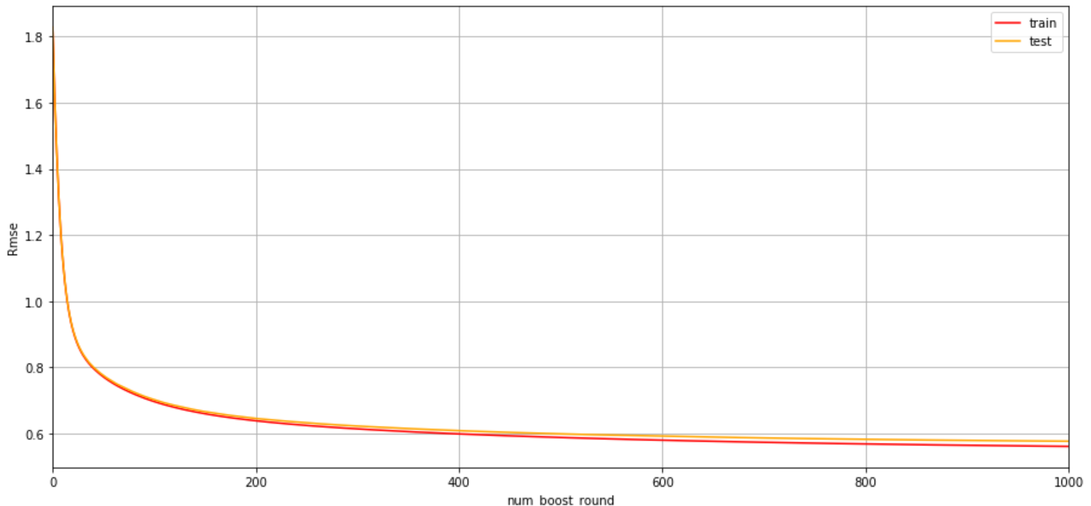
# 绘制误差曲线
plt.figure(figsize=(15, 7))
plt.grid()
plt.plot(range(0, len(cv_result['train-rmse-mean'])),
         cv_result['train-rmse-mean'], c='red', label='train')
plt.plot(range(0, len(cv_result['test-rmse-mean'])),
         cv_result['test-rmse-mean'], c='orange', label='test')
plt.xlabel('num_boost_round')
plt.ylabel('Rmse')
plt.xlim((0, num_boost_round))
plt.legend()
plt.show()
2、sklearn API
官方文档:Using the Scikit-Learn Estimator Interface — xgboost 2.1.0-dev documentation
二分类
X, y = load_digits(n_class=2, return_X_y=True)

X_train, X_test, y_train, y_test = train_test_split(X, y, test_size=0.2)
# 参数设置
bst_sk = xgb.XGBClassifier(
    n_estimators = 50,
    max_depth = 2,
    objective = 'binary:logistic',
    eval_metric = "error",
    early_stopping_rounds = 5
)

# 模型训练
bst_sk.fit(X_train, y_train, eval_set=[(X_test, y_test)])

# 预测结果
preds_sk = bst_sk.predict(X_test)

# 预测准确度
print('--'*25)
print(f"预测准确度:{accuracy_score(y_test, preds_sk):.3f}")

# 混淆矩阵
print('--'*25)
print("混淆矩阵:")
print(confusion_matrix(y_test, preds_sk))
[0]	validation_0-error:0.00000
[1]	validation_0-error:0.00000
[2]	validation_0-error:0.01389
[3]	validation_0-error:0.01389
[4]	validation_0-error:0.00000
[5]	validation_0-error:0.01389
--------------------------------------------------
预测准确度:1.000
--------------------------------------------------
混淆矩阵:
[[36  0]
 [ 0 36]]
多分类
X, y = load_digits(n_class=10, return_X_y=True)

X_train, X_test, y_train, y_test = train_test_split(X, y, test_size=0.2)
# 训练模型
bst_sk = xgb.XGBClassifier(
        n_estimators = 100,
        max_depth = 2,
        learning_rate = 0.8,
        verbosity = 0,
        objective = "multi:softmax",
        booster = 'gbtree',
        tree_method = 'hist',
        max_bins = 256,
        gamma = 0,
        subsample = 1,
        colsample_bytree = 1,
        colsample_bylevel = 1,
        colsample_bynode = 1,
        reg_alpha = 0,
        reg_lambda = 1,
        eval_metric = "merror",
        early_stopping_rounds = 10
    )

bst_sk.fit(X_train, y_train, eval_set=[(X_test, y_test)])

# 预测结果
preds_sk = bst_sk.predict(X_test, iteration_range=(0, bst_sk.best_iteration + 1))

# 预测准确度
print('--'*25)
print(f"预测准确度:{accuracy_score(y_test, preds_sk):.3f}")

# 混淆矩阵
print('--'*25)
print("混淆矩阵:")
print(confusion_matrix(y_test, preds_sk))
[0]	validation_0-merror:0.26111
[1]	validation_0-merror:0.19167
[2]	validation_0-merror:0.16389
[3]	validation_0-merror:0.13333
[4]	validation_0-merror:0.11667
[5]	validation_0-merror:0.10000
[6]	validation_0-merror:0.08611
[7]	validation_0-merror:0.07500
[8]	validation_0-merror:0.07222
[9]	validation_0-merror:0.06944
[10]	validation_0-merror:0.05833
[11]	validation_0-merror:0.05833
[12]	validation_0-merror:0.05556
[13]	validation_0-merror:0.06111
[14]	validation_0-merror:0.05833
[15]	validation_0-merror:0.05833
[16]	validation_0-merror:0.06111
[17]	validation_0-merror:0.06111
[18]	validation_0-merror:0.05833
[19]	validation_0-merror:0.06111
[20]	validation_0-merror:0.05833
[21]	validation_0-merror:0.05833
[22]	validation_0-merror:0.05833
--------------------------------------------------
预测准确度:0.944
--------------------------------------------------
混淆矩阵:
[[37  0  0  0  0  0  0  0  0  0]
 [ 0 33  1  1  0  0  0  0  0  2]
 [ 1  1 34  2  0  0  0  0  0  1]
 [ 0  0  0 30  0  0  0  1  0  0]
 [ 0  1  0  0 36  0  0  0  0  0]
 [ 0  0  0  0  0 35  0  0  1  2]
 [ 0  0  0  0  0  0 45  0  0  0]
 [ 0  0  0  1  0  0  0 33  0  1]
 [ 0  2  0  1  0  0  0  1 31  0]
 [ 0  0  0  0  0  0  0  0  0 26]]
回归
# 导入数据集,并拆分为训练集和测试集
X, y = fetch_california_housing(return_X_y=True)
X_train, X_test, y_train, y_test = train_test_split(X, y, test_size=0.2, shuffle=True)
# 训练模型
model = xgb.XGBRegressor(
n_estimators = 1000,
learing_rate = 0.1,
gamma = 0,
max_depth = 1,
booster = 'gbtree',
objective = 'reg:squarederror',
eval_metric = ['rmse'],
early_stopping_rounds = 10,
verbosity = 1
)
model.fit(X_train, y_train, eval_set=[(X_train, y_train), (X_test, y_test)])
# 训练和测试结果
train_rmse = model.evals_result_['validation_0']['rmse']
test_rmse = model.evals_result_['validation_1']['rmse']
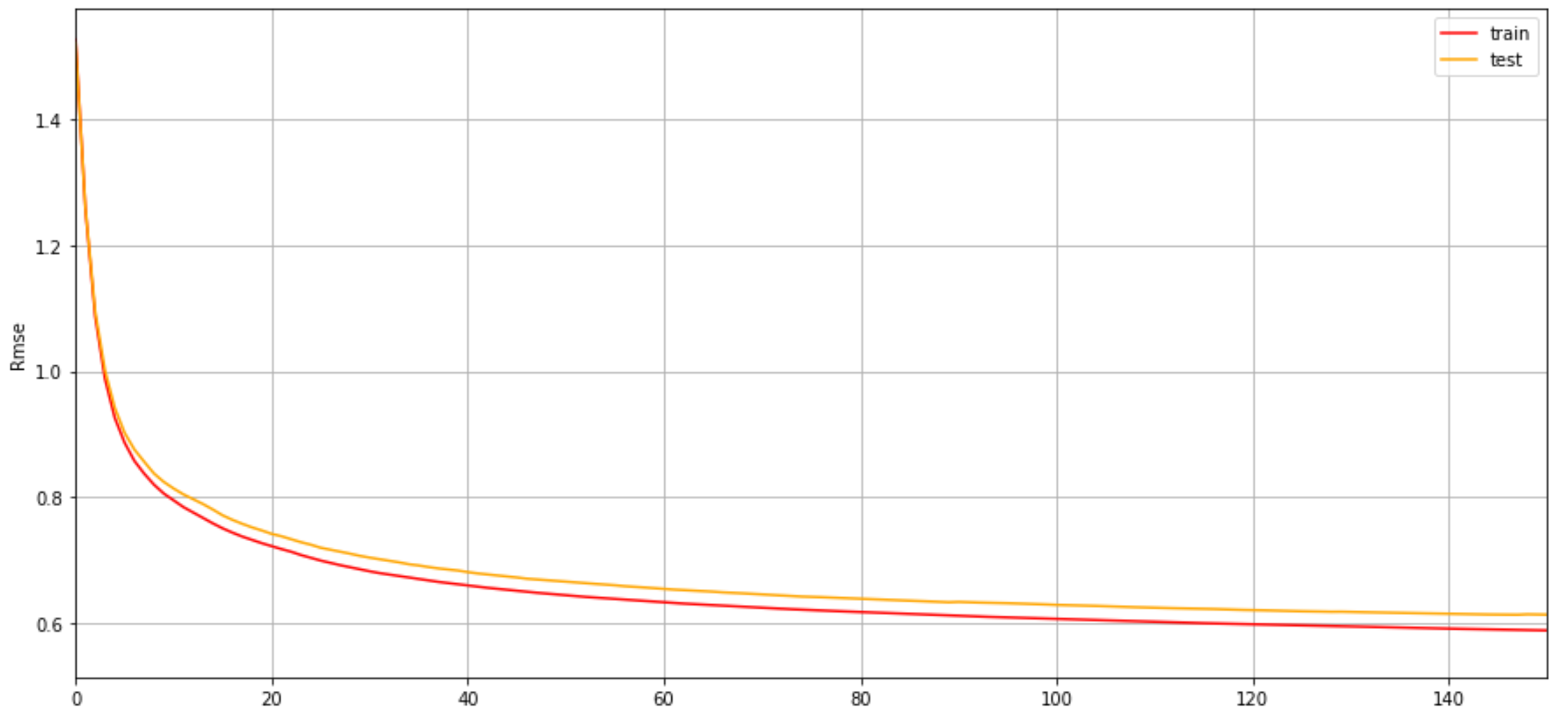
# 绘制误差曲线
plt.figure(figsize=(15, 7))
plt.grid()
plt.plot(range(0, len(train_rmse)),
train_rmse, c='red', label='train')
plt.plot(range(0, len(test_rmse)),
test_rmse, c='orange', label='test')
plt.xlabel('Steps')
plt.ylabel('Rmse')
plt.xlim((0, 150))
plt.legend()
plt.show()


 浙公网安备 33010602011771号