决策树模型系列——6、集成学习技术框架_Stacking算法

在scikit-learn中提供了两种统一的Stacking methods，分类器StackingClassifier和回归器StackingRegressor，初级学习器estimators和次级学习器final_estimator可以是用户自己定义的，可以是决策树、KNN、SVM、深度学习网络等，最后通过Stacking方法将各初级学习器的输出结果作为次级学习的输入，最后由次级学习器输出预测结果。

Scikit-learn使用案例

import numpy as np

from sklearn.datasets import fetch_openml
from sklearn.utils import shuffle
from sklearn.compose import make_column_selector, make_column_transformer
from sklearn.impute import SimpleImputer
from sklearn.pipeline import make_pipeline
from sklearn.preprocessing import OrdinalEncoder, OneHotEncoder, StandardScaler
from sklearn.linear_model import LassoCV, RidgeCV
from sklearn.ensemble import RandomForestRegressor, HistGradientBoostingRegressor, StackingRegressor
from sklearn.model_selection import cross_validate, cross_val_predict

import time

import matplotlib.pyplot as plt

def load_ames_housing():
    """从OpenML提取Ames Housing数据集
    （该数据集有1460个样本，80个特征）"""
    df = fetch_openml(name='house_prices', as_frame=True)
    X = df.data   #特征值
    y = df.target #目标值
    
    # 提取其中20个比较感兴趣的特征数据
    features = [
        "YrSold",
        "HeatingQC",
        "Street",
        "YearRemodAdd",
        "Heating",
        "MasVnrType",
        "BsmtUnfSF",
        "Foundation",
        "MasVnrArea",
        "MSSubClass",
        "ExterQual",
        "Condition2",
        "GarageCars",
        "GarageType",
        "OverallQual",
        "TotalBsmtSF",
        "BsmtFinSF1",
        "HouseStyle",
        "MiscFeature",
        "MoSold",
    ]
    
    X = X.loc[:, features]
    X, y = shuffle(X, y, random_state=0)  #随机打乱数据
    
    # 提取其中600个数据
    X = X.iloc[:600]
    y = y.iloc[:600]
    
    return X, np.log(y)

# 使用pipeline预处理数据
# 分类类型选择器
cat_selector = make_column_selector(dtype_include=object)
# 数值类型选择器
num_selector = make_column_selector(dtype_include=np.number)

# 树模型的数据预处理转换器
# 分类型变量用顺序型编码OrdinalEncoder
cat_tree_processor = OrdinalEncoder(
    handle_unknown = "use_encoded_value",
    unknown_value = -1
)

# 连续型变量设置一个简单处理器SimpleImputer进行处理
num_tree_processor = SimpleImputer(
    strategy = 'mean',
    add_indicator = True
)

# 变量转换器
tree_preprocessor = make_column_transformer(
    (num_tree_processor, num_selector),
    (cat_tree_processor, cat_selector)
)

print(tree_preprocessor)

# 线性模型的数据预处理转换器
cat_linear_processor = OneHotEncoder(handle_unknown='ignore')
num_linear_processor = make_pipeline(
    StandardScaler(),
    SimpleImputer(strategy='mean', add_indicator=True)
)
linear_preprocessor = make_column_transformer(
    (num_linear_processor, num_selector),
    (cat_linear_processor, cat_selector)
)
print(linear_preprocessor)

# LassoCV模型
lasso_pipeline = make_pipeline(linear_preprocessor, LassoCV())
print(lasso_pipeline)

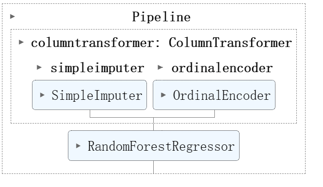
# RF
rf_pipeline = make_pipeline(
    tree_preprocessor,
    RandomForestRegressor(random_state=42)
)
print(rf_pipeline)

#HGBR
gbdt_pipeline = make_pipeline(
    tree_preprocessor,
    HistGradientBoostingRegressor(random_state=0)
)
print(gbdt_pipeline)

# Stacking
estimators = [
    ('Random Forest', rf_pipeline),
    ('Lasso', lasso_pipeline),
    ('Gradient Boosting', gbdt_pipeline)
]

stacking_regressor = StackingRegressor(
    estimators = estimators,
    final_estimator = RidgeCV()
)

print(stacking_regressor)

def plot_regression_results(ax, y_true, y_pred, title, scores, elapsed_time):
    """实际值和预测值的散点对比图"""
    ax.plot(
        [y_true.min(), y_true.max()],
        [y_true.min(), y_true.max()],
        '--r', linewidth=2
    )
    ax.scatter(y_true, y_pred, alpha=0.2)
    
    ax.spines['top'].set_visible(False)
    ax.spines['right'].set_visible(False)
    ax.get_xaxis().tick_bottom()
    ax.get_yaxis().tick_left()
    ax.spines['left'].set_position(('outward', 10))
    ax.spines['bottom'].set_position(('outward', 10))
    ax.set_xlim([y_true.min(), y_true.max()])
    ax.set_ylim([y_true.min(), y_true.max()])
    ax.set_xlabel('Measured')
    ax.set_ylabel('Predicted')
    extra = plt.Rectangle(
        (0, 0), 0, 0, fc='w', fill=False,
        edgecolor='none', linewidth=0
    )
    ax.legend([extra], [scores], loc='upper left')
    title = title + '\n Evaluation in {:.2f} seconds'.format(elapsed_time)
    ax.set_title(title)

fig, axes = plt.subplots(2, 2, figsize=(12, 6))
axes = np.ravel(axes)

for ax, (name, est) in zip(axes, estimators + [('Stacking Regressor', stacking_regressor)]):
    start_time = time.time()
    score = cross_validate(
        est, X, y, scoring=['r2', 'neg_mean_absolute_error'],
        n_jobs=-1, verbose=0
    )
    elapsed_time = time.time() - start_time
    
    y_pred = cross_val_predict(est, X, y, n_jobs=-1, verbose=0)
    
    plot_regression_results(
        ax, y, y_pred, name,
        (f"$R^2={np.mean(score['test_r2']):.2f} \pm {np.std(score['test_r2']):.2f}$" 
         + "\n" + f"$MAE={-np.mean(score['test_neg_mean_absolute_error']):.2f} \pm {np.std(score['test_neg_mean_absolute_error']):.2f}$"),
        elapsed_time,
    )

plt.suptitle('Single predictions versus stacked predictors')
plt.tight_layout()
plt.subplots_adjust(top=0.9)
plt.show()

$ $
参考资料

1. https://scikit-learn.org/stable/modules/ensemble.html#stacked-generalization