

1 基于阈值
灰度阈值法,是最简单、速度最快的图像分割方法,广泛用于实时图像处理领域 ,尤其是嵌入式系统中
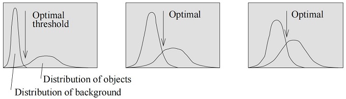
设输入图像 $f$,输出图像 $g$,则阈值化公式为 $ \begin{equation} g(i, j) = \begin{cases}1, &\text{f(i, j) ≥ T} \\ 0, &\text{f(i, j) < T} \end{cases} \end{equation}$
通俗说,就是遍历图像中的像素,当像素值 $f (i, j) ≥ T$ 时,标记 $g (i, j)$ 为物体像素,否则为背景像素
当各物体不接触,且在图像中 物体和背景的灰度值差别比较明显 时,阈值法是非常合适的分割方法
1.1 固定阈值
固定阈值化函数为 threshold(),如下:
double threshold (
    InputArray    src,   // 输入图像 (单通道,8位或32位浮点型)
    OutputArray   dst,   // 输出图像 (大小和类型,同输入)
    double    thresh,   // 阈值
    double    maxval,   // 最大灰度值(使用 THRESH_BINARY 和 THRESH_BINARY_INV类型时)
    int        type    // 阈值化类型(THRESH_BINARY, THRESH_BINARY_INV; THRESH_TRUNC; THRESH_TOZERO, THRESH_TOZERO_INV)
)
不同的阈值化类型对应的公式,如下:
1) THRESH_BINARY
$\qquad dst(x, y) = \begin{cases} maxval & \text{if src(x, y) > thresh} \\0 & \text{otherwise} \\ \end{cases} $
2) THRESH_TRUNC
$\qquad dst(x, y) = \begin{cases} threshold & \text{if src(x, y) > thresh} \\src(x, y) & \text{otherwise} \\ \end{cases} $
3) THRESH_TOZERO
$\qquad dst(x, y) = \begin{cases} src(x, y) & \text{if src(x, y) > thresh} \\0 & \text{otherwise} \\ \end{cases} $
1.2 自适应阈值
整幅图像使用同一个阈值做二值化,对于一些情况并不适用,尤其是当图像中的不同区域,照明条件各不相同时。此时,需要自适应阈值算法
该算法可根据像素所在的区域,确定一个适合的阈值,对于一幅图中光照不同的区域,可取各自不同的阈值做二值化
目前有 MEAN_C 和 GAUSSIAN_C 两种算法,OpenCV 中的自适应阈值化函数为 adaptiveThreshold(),如下:
void  adaptiveThreshold (
    InputArray          src,   //
    OutputArray         dst,   //
    double         maxValue,   //
    int      adaptiveMethod,   // 自适应阈值算法
    int       thresholdType,   // 阈值化类型,同 threshold() 中的 type
    int           blockSize,   // 邻域大小
    double                C    //
)
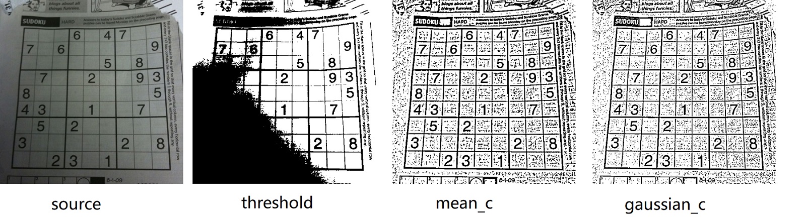
1.3 示例
全局阈值和自适应阈值的比较,代码如下:
#include "opencv2/imgproc.hpp"
#include "opencv2/highgui.hpp"

using namespace cv;

int main()
{
    // read an image
    Mat img = imread("sudoku.png", IMREAD_GRAYSCALE);

    // adaptive
    Mat dst1, dst2, dst3;
    threshold(img, dst1, 100, 255, THRESH_BINARY);
    adaptiveThreshold(img, dst2, 255, ADAPTIVE_THRESH_MEAN_C, THRESH_BINARY, 11, 2);
    adaptiveThreshold(img, dst3, 255, ADAPTIVE_THRESH_GAUSSIAN_C, THRESH_BINARY, 11, 2);

    // ... ...
    waitKey();
}
对比结果如下:
2 基于边缘
OpenCV 之 边缘检测 中,介绍了三种边缘检测算子: Sobel,Laplace 和 Canny 算子
但边缘检测的结果是离散的点,不能作为图像分割的结果,必须将边缘点沿着图像的边界连接起来,形成边缘链
2.1 轮廓函数
OpenCV 中,可在图像的边缘检测之后,使用 findContours() 寻找到轮廓,该函数参数如下:
image 一般为二值化图像,可由 compare, inRange, threshold , adaptiveThreshold, Canny 等函数获得
void findContours (
    InputOutputArray         image,   // 输入图像
    OutputArrayOfArrays   contours,   // 检测到的轮廓
    OutputArray          hierarchy,   // 可选的输出向量
    int                 mode,         // 轮廓获取模式 (RETR_EXTERNAL, RETR_LIST, RETR_CCOMP,RETR_TREE, RETR_FLOODFILL)
    int               method,         // 轮廓近似算法 (CHAIN_APPROX_NONE, CHAIN_APPROX_SIMPLE, CHAIN_APPROX_TC89_L1, CHAIN_APPROX_TC89_KCOS)
    Point    offset = Point()         // 轮廓偏移量
)
hierarchy 为可选的参数,如果不选择该参数,则可得到 findContours 函数的第二种形式
void findContours (
  InputOutputArray   image,
  OutputArrayOfArrays contours,
  int    mode,
  int    method,
  Point   offset = Point()
)
drawContours() 函数如下:
void drawContours (
    InputOutputArray            image,     // 目标图像
    InputArrayOfArrays       contours,     // 所有的输入轮廓
    int                   contourIdx,     //
    const Scalar &              color,     //  轮廓颜色
    int                 thickness = 1,     //  轮廓线厚度
    int             lineType = LINE_8,     //
    InputArray  hierarchy = noArray(),     //
    int            maxLevel = INT_MAX,     //
    Point             offset = Point()     //
)
2.2 例程
代码摘自 OpenCV 例程,略有修改
#include "opencv2/imgcodecs.hpp"
#include "opencv2/highgui.hpp"
#include "opencv2/imgproc.hpp"

using namespace cv;
using namespace std;

Mat src,src_gray;
int thresh = 100;
int max_thresh = 255;
RNG rng(12345);

void thresh_callback(int, void* );

int main( int, char** argv )
{
  // 读图
  src = imread("Pillnitz.jpg", IMREAD_COLOR);
  if (src.empty())
      return -1;

  // 转化为灰度图
  cvtColor(src, src_gray, COLOR_BGR2GRAY );
  blur(src_gray, src_gray, Size(3,3) );

  // 显示
  namedWindow("Source", WINDOW_AUTOSIZE );
  imshow( "Source", src );

  // 滑动条
  createTrackbar("Canny thresh:", "Source", &thresh, max_thresh, thresh_callback );

  // 回调函数
  thresh_callback( 0, 0 );

  waitKey();
}

// 回调函数
void thresh_callback(int, void* )
{
  Mat canny_output;
  vector<vector<Point> > contours;
  vector<Vec4i> hierarchy;

  // 边缘检测 + 轮廓
  Canny(src_gray, canny_output, thresh, thresh*2, 3);
  findContours( canny_output, contours, hierarchy, RETR_TREE, CHAIN_APPROX_SIMPLE, Point(0, 0) );

  // 画轮廓
  Mat drawing = Mat::zeros( canny_output.size(), CV_8UC3);
  for( size_t i = 0; i< contours.size(); i++ ) {
      Scalar color = Scalar( rng.uniform(0, 255), rng.uniform(0,255), rng.uniform(0,255) );
      drawContours( drawing, contours, (int)i, color, 2, 8, hierarchy, 0, Point() );
  }
  namedWindow( "Contours", WINDOW_AUTOSIZE );
  imshow( "Contours", drawing );
}
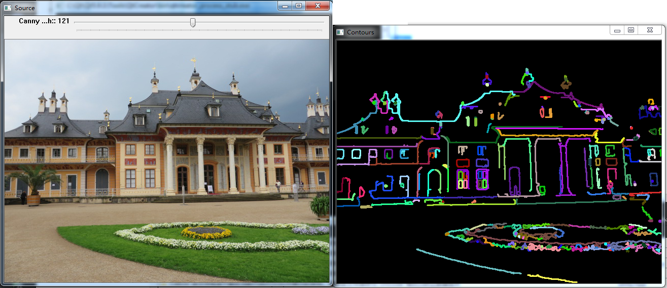
以 Dresden 的 Schloss Pillnitz 为源图,输出如下:
参考资料
OpenCV Tutorials / imgproc module / Basic Thresholding Operations
OpenCV Tutorials / imgproc module / Finding contours in your image
OpenCV-Python Tutorials / Image Processing in OpenCV / Image Thresholding
《Image Processing, Analysis, and Machine Vision》4th,ch6
Topological structural analysis of digitized binary images by border following [J], Satoshi Suzuki, 1985
更新记录
2020年4月26日,增加 “1.3 自适应阈值化” 和 “1.4 示例 - 自适应阈值代码”
原文链接: http://www.cnblogs.com/xinxue/
专注于机器视觉、OpenCV、C++ 编程

