Deeplearning.ai-Course-2-浅层神经网络(编程作业)
声明:本文参考https://blog.csdn.net/u013733326/article/details/79702148,记录学习过程中的心得体会
Python版本:3.6.x
实验目的:搭建一个能分类平面数据的浅层神经网络,它只有一个隐藏层
在这篇文章中,我们会学到以下知识:
- 构建具有单隐藏层的二分类神经网络
- 了解非线性激活函数,如tanh函数
- 计算损失函数
- 编程实现前向传播和后向传播
实验步骤:
一、加载、处理数据
开始前引入的库:


import numpy as np
import matplotlib.pyplot as plt
import sklearn
import sklearn.datasets
import sklearn.linear_model
from testCases import *
from planar_utils import plot_decision_boundary, sigmoid, load_planar_dataset, load_extra_datasets
- sklearn:进行数据挖掘和数据分析的框架
- testCases:提供一些测试样例评估函数的正确性
- planar_utils:提供在本实验中使用的功能函数
加载、查看数据集:
X, Y = load_planar_dataset()
plt.scatter(X[0,:], X[1,:], c = np.squeeze(Y), s = 40, cmap = plt.cm.Spectral) #s表示大小,c表示颜色序列,cmap表示Colormap
plt.show()

shape_X = X.shape #(2,400)
shape_Y = Y.shape #(1,400)
m = Y.shape[1]   #训练集里面的数量
print ("X的维度为: " + str(shape_X))
print ("Y的维度为: " + str(shape_Y))
print ("数据集里面的数据有:" + str(m) + " 个")

X的维度为: (2, 400)
Y的维度为: (1, 400)
数据集里面的数据有:400 个
符号说明:
- X:(2,400)的numpy矩阵,包含数据点的数值
- Y:(1,400)的numpy向量,对应X的标签(0-red、1-blue)
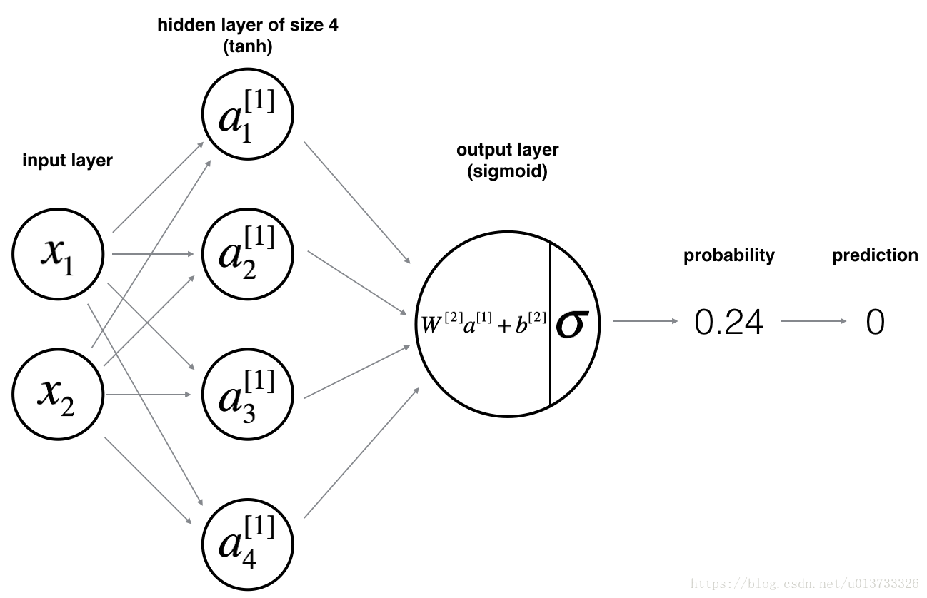
二、搭建浅层神经网络
浅层神经网路的模型如下图:
前向传播:
对单个样本$\left \{ x^{\left ( i \right )},y^{\left ( i \right )}\right \}$:
隐藏层中每个神经元的计算过程如下:
$$\left\{\begin{matrix}
z_{1}^{\left [ 1 \right ]}=w_{1}^{\left [ 1 \right ]}x + b_{1}^{\left [ 1 \right ]} &a_{1}^{\left [ 1 \right ]}=\sigma \left ( z_{1}^{\left [ 1 \right ]} \right ) \\
z_{2}^{\left [ 1 \right ]}=w_{2}^{\left [ 1 \right ]}x + b_{2}^{\left [ 1 \right ]} &a_{2}^{\left [ 1 \right ]}=\sigma \left ( z_{2}^{\left [ 1 \right ]} \right )\\
z_{3}^{\left [ 1 \right ]}=w_{3}^{\left [ 1 \right ]}x + b_{3}^{\left [ 1 \right ]} &a_{3}^{\left [ 1 \right ]}=\sigma \left ( z_{3}^{\left [ 1 \right ]} \right ) \\
z_{4}^{\left [ 1 \right ]}=w_{4}^{\left [ 1 \right ]}x + b_{4}^{\left [ 1 \right ]} &a_{4}^{\left [ 1 \right ]}=\sigma \left ( z_{4}^{\left [ 1 \right ]} \right )
\end{matrix}\right.$$
$$\begin{align*}
z^{\left [ 1 \right ]}&=\begin{bmatrix}
z_{1}^{\left [ 1 \right ]}\\
z_{2}^{\left [ 1 \right ]}\\
z_{3}^{\left [ 1 \right ]}\\
z_{4}^{\left [ 1 \right ]}
\end{bmatrix}=\begin{bmatrix}
\cdots &W_{1}^{\left [ 1 \right ]T} & \cdots \\
\cdots &W_{2}^{\left [ 1 \right ]T} & \cdots \\
\cdots &W_{3}^{\left [ 1 \right ]T} &\cdots \\
\cdots &W_{4}^{\left [ 1 \right ]T} & \cdots
\end{bmatrix}\ast \begin{bmatrix}
x_{1}\\x_{2}
\end{bmatrix}+\begin{bmatrix}
b_{1}^{\left [ 1 \right ]}\\
b_{2}^{\left [ 1 \right ]}\\
b_{3}^{\left [ 1 \right ]}\\
b_{4}^{\left [ 1 \right ]}
\end{bmatrix}\\\\
z^{\left [ 1 \right ]}&=W^{\left [ 1 \right ]}x+b^{\left [ 1 \right ]}
\end{align*}$$
$$a^{\left [ 1 \right ]}=\begin{bmatrix}
a_{1}^{\left [ 1 \right ]}\\
a_{2}^{\left [ 1 \right ]}\\
a_{3}^{\left [ 1 \right ]}\\
a_{4}^{\left [ 1 \right ]}
\end{bmatrix}=\sigma \left ( \begin{bmatrix}
z_{1}^{\left [ 1 \right ]}\\
z_{2}^{\left [ 1 \right ]}\\
z_{3}^{\left [ 1 \right ]}\\
z_{4}^{\left [ 1 \right ]}
\end{bmatrix} \right )=\sigma \left ( z^{\left [ 1 \right ]} \right )$$
对于多个样本
$$X = \begin{bmatrix}
\vdots & \vdots & \vdots & \vdots \\
x^{\left ( 1 \right )} & x^{\left ( 2 \right )} & \cdots &x^{\left ( m \right )} \\
\vdots & \vdots & \vdots & \vdots
\end{bmatrix}$$
对于所有训练样本,需要让i从1到m实现下式:
$$z^{\left [ 1 \right ]\left ( i \right )}=W^{\left [ 1 \right ]}x^{\left ( i \right )}+b^{\left [ 1 \right ]}\\$$
$$a^{\left [ 1 \right ]\left ( i \right )}=\sigma \left ( z^{\left [ 1 \right ]\left ( i \right )} \right )$$
所以有
$$\begin{align*}
Z^{\left [ 1 \right ]} &= \begin{bmatrix}
\vdots & \vdots & \vdots & \vdots \\
z^{\left [ 1 \right ]\left ( 1 \right )} & z^{\left [ 1 \right ]\left ( 2 \right )} & \cdots &z^{\left [ 1 \right ]\left ( m \right )} \\
\vdots & \vdots & \vdots & \vdots
\end{bmatrix}\\&=\begin{bmatrix}
W^{\left [ 1 \right ]}x^{\left ( 1 \right )}+b^{\left [ 1 \right ]} &W^{\left [ 1 \right ]}x^{\left ( 2\right )}+b^{\left [ 1 \right ]} &\cdots & W^{\left [ 1 \right ]}x^{\left ( m \right )}+b^{\left [ 1 \right ]}
\end{bmatrix}\\&=W^{\left [ 1 \right ]}\begin{bmatrix}
x^{\left ( 1 \right )}&x^{\left ( 2\right )} &\cdots & x^{\left ( m \right )}
\end{bmatrix} +\begin{bmatrix}
b^{\left [ 1 \right ]} & b^{\left [ 1 \right ]} & \cdots & b^{\left [ 1 \right ]}
\end{bmatrix}\\&=W^{\left [ 1 \right ]}X+b^{\left [ 1 \right ]}(Python中的广播机制)
\end{align*}$$
$$\begin{align*}
A^{\left [ 1 \right ]}&=\begin{bmatrix}
\vdots &\vdots & \vdots &\vdots \\
a^{\left [ 1 \right ]\left ( 1 \right )}& a^{\left [ 1 \right ]\left ( 2 \right )} & \cdots & a^{\left [ 1 \right ]\left ( m \right )} \\
\vdots & \vdots &\vdots & \vdots
\end{bmatrix}=\begin{bmatrix}
\sigma \left ( z^{\left [ 1 \right ]\left ( 1 \right )} \right )& \sigma \left ( z^{\left [ 1 \right ]\left ( 2 \right )} \right ) &\cdots & \sigma \left ( z^{\left [ 1 \right ]\left ( m \right )} \right )
\end{bmatrix}\\&=\sigma \begin{bmatrix}
z ^{\left [ 1 \right ]\left ( 1 \right )}&z ^{\left [ 1 \right ]\left ( 2 \right )} &\cdots & z ^{\left [ 1 \right ]\left ( m \right )}
\end{bmatrix}=\sigma\left ( Z^{\left [ 1 \right ]} \right )
\end{align*}$$
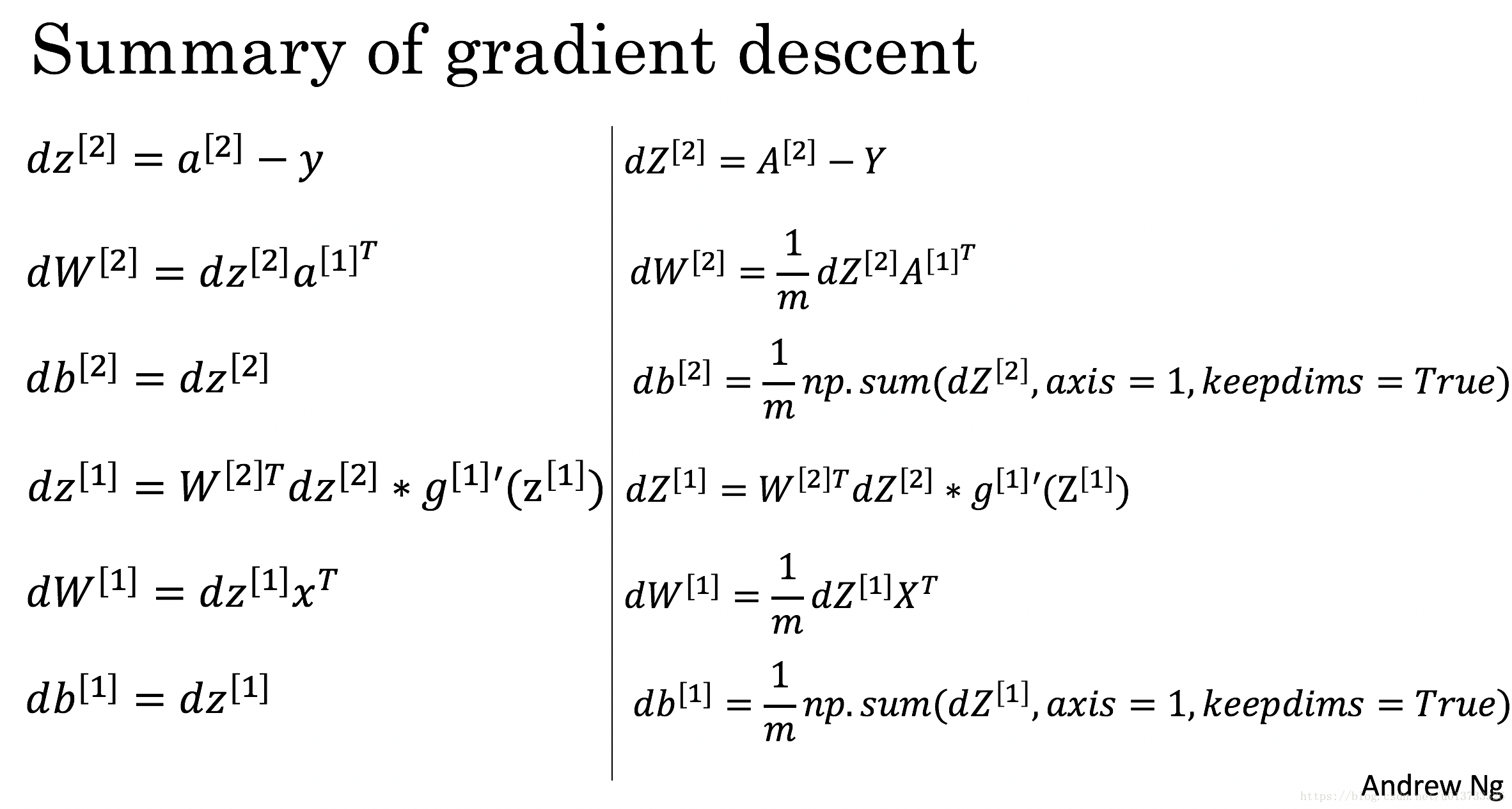
反向传播
对于单个样例$\left \{ x,y \right \}$(省略上标):
$$\because z^{\left [ 2 \right ]}=W^{\left [ 2 \right ]}a^{\left [ 1 \right ]}+b^{\left [ 2 \right ]}\\$$
$$a^{\left [ 2 \right ]}=\sigma \left ( z^{\left [ 2 \right ]} \right )\\$$
$$\therefore dz^{\left [ 2 \right ]}=a^{\left [ 2 \right ]}-y\\$$
$$db^{\left [ 2 \right ]}=dz^{\left [ 2 \right ]}\\$$
$$dW^{\left [ 2 \right ]}=dz^{\left [ 2 \right ]}a^{\left [ 1 \right ]T}\Leftrightarrow \left ( n^{\left [ 2 \right ]},n^{\left [ 1 \right ]}\right )= \left ( n^{\left [ 2 \right ]} ,1 \right )*\left (1,n^{\left [ 1 \right ]}\right)\\$$
$$da^{\left [ 1 \right ]}=W^{\left [ 2 \right ]T}dz^{\left [ 2 \right ]}\Leftrightarrow \left ( n^{\left [ 1 \right ]},1 \right )=\left ( n^{\left [ 1 \right ]},n^{\left [ 2 \right ]} \right )*\left ( n^{\left [ 2 \right ]} ,1\right )\\$$
$$\because z^{\left [ 1 \right ]}=W^{\left [ 1 \right ]}a^{\left [ 0 \right ]}+b^{\left [ 1 \right ]}\left(a^{\left [ 0 \right ]}=x \right )\\$$
$$a^{\left [ 1 \right ]}=g^{\left [ 1 \right ]}\left ( z^{\left [ 1 \right ]} \right )\\$$
$$dz^{\left [ 1 \right ]}=da^{\left [ 1 \right ]}\ast g^{\left [ 1 \right ]}{}'\left ( z^{\left [ 1 \right ]} \right )=W^{\left [ 2 \right ]T}dz^{\left [ 2 \right ]}\ast g^{\left [ 1 \right ]}{}'\left ( z^{\left [ 1 \right ]} \right )\\$$
$$db^{\left [ 1 \right ]}=dz^{\left [ 1 \right ]}\\$$
$$dW^{\left [ 1 \right ]}=dz^{\left [ 1 \right ]}a^{\left [ 0 \right ]T}=dz^{\left [ 1 \right ]}x$$
对于全部样例$\left \{ X,Y \right \}$:
$$A^{\left [ 2 \right ]}=\begin{bmatrix}
\vdots & \vdots &\vdots &\vdots \\
a^{\left [ 2 \right ]\left ( 1 \right )}& a^{\left [ 2 \right ]\left ( 2 \right )} & \cdots &a^{\left [ 2 \right ]\left ( m \right )} \\
\vdots&\vdots & \vdots &\vdots
\end{bmatrix}\\$$
$$Y=\begin{bmatrix}
y^{\left ( 1 \right )} & y^{\left ( 2 \right )} & \cdots & y^{\left ( m \right )}
\end{bmatrix}\\$$
$$\begin{align*}
dZ^{\left [ 2 \right ]}&=\begin{bmatrix}
dz^{\left [ 2 \right ]\left ( 1 \right )}& dz^{\left [ 2 \right ]\left ( 2 \right )} & \cdots & dz^{\left [ 2 \right ]\left ( m \right )}
\end{bmatrix}\\&=\begin{bmatrix}
a^{\left [ 2 \right ]\left ( 1 \right )}-y^{\left ( 1 \right )} & a^{\left [ 2 \right ]\left ( 2 \right )}-y^{\left ( 2 \right )} &\cdots & a^{\left [ 2 \right ]\left ( m \right )}-y^{\left ( m\right )}
\end{bmatrix}\\ &=A^{\left [ 2 \right ]}-Y
\end{align*}$$
全部样例对W1的偏导数实际上是从1到m所有单个样例对W1偏导数的平均值:
$$\begin{align*}
dW^{\left [ 2 \right ]}&=\frac{1}{m}\sum_{i=1}^{m}dz^{\left [ 2 \right ]\left ( i \right )}a^{\left [ 1 \right ]\left ( i \right )T}=\frac{1}{m}\begin{bmatrix}
dz^{\left [ 2 \right ]\left ( 1 \right )}&\cdots & dz^{\left [ 2 \right ]\left ( m \right )}
\end{bmatrix}\begin{bmatrix}
a^{\left [ 1 \right ]\left ( 1 \right )T}\\
\cdots \\ a^{\left [ 1 \right ]\left ( m \right )T}
\end{bmatrix}\\
&=\frac{1}{m}\begin{bmatrix}
dz^{\left [ 2 \right ]\left ( 1 \right )} &\cdots & dz^{\left [ 2 \right ]\left ( m \right )}
\end{bmatrix}\begin{bmatrix}
a^{\left [ 1 \right ]\left ( 1 \right )} & \cdots &a^{\left [ 1 \right ]\left ( m \right )}
\end{bmatrix}^{T}=\frac{1}{m}np.dot\left ( dZ^{\left [ 2 \right ]},A^{\left [ 1 \right ]T} \right )
\end{align*}$$
$$db^{\left [ 2 \right ]}=\frac{1}{m}\sum_{i=1}^{m}dz^{\left [ 2 \right ]\left ( i \right )}=\frac{1}{m}np.sum\left ( dZ^{\left [ 2 \right ]},axis=1,keepdims=True \right )$$
注:axis=1,表示按照行取平均值
单个样例和全部样例的公式表格如下:
三、搭建神经网络的一般方法
- 定义神经网络的结构(输入单元的数量,隐藏层的单元数量等)
- 初始化神经网络的参数
- LOOP
- 前向传播
- 计算损失函数
- 反向传播
- 更新参数(梯度下降)
1、定义神经网络的结构
- n_x:输入层的数量
- n_h:隐藏层的数量(这里定义为4)
- n_y:输出层的数量
def layer_sizes(X, Y):
    """
        n_x - 输入层的数量
        n_h - 隐藏层的数量
        n_y - 输出层的数量
    """
    n_x = X.shape[0]
    n_h = 4
    n_y = Y.shape[0]

    return (n_x, n_h, n_y)
2、初始化神经网络的参数
- 采用随机值初始化权重矩阵,np.random.randn(a,b) *0.01 来随机初始化一个维度为(a,b)的矩阵。
numpy.random.rand(a,b) #将根据给定维度生成[0,1)之间的数据,包含0,不包含1
numpy.random.randn(a,b) #生成的数据符合标准正态分布,均值为0,标准差为1
- 将偏向量初始化为零,np.zeros((a,b)) ,注意是两个括号
def initialize_parameters(n_x, n_h, n_y):
    """
    return:
         parameters - 包含参数的字典
         W1 - 权重矩阵, 维度(n_h, n_x)
         b1 - 偏置向量, 维度(n_h, 1)
         W2 - 权重矩阵, 维度(n_y, n_h)
         b2 - 偏置向量, 维度(n_y, 1)
    """
    np.random.seed(2)
    W1 = np.random.randn(n_h, n_x) * 0.01
    b1 = np.zeros(shape = (n_h, 1))
    W2 = np.random.randn(n_y, n_h) * 0.01
    b2 = np.zeros(shape = (n_y, 1))

    # 使用断言确保我的数据格式是正确的
    assert (W1.shape == (n_h, n_x))
    assert (b1.shape == (n_h, 1))
    assert (W2.shape == (n_y, n_h))
    assert (b2.shape == (n_y, 1))

    parameters = {"W1" : W1, "b1" : b1, "W2" : W2, "b2" : b2}
    return parameters
3、LOOP
前向传播
步骤如下:
- 使用字典类型的parameters(它是initialize_parameters() 的输出)检索每个参数
-
实现前向传播,计算训练集所有样例的预测向量
- 将反向传播所需要的值存储在cache中
def forward_propagation(X, parameters):
    """
    :param X - 维度(n_x,m)的输入数据
    :param parameters - 初始化函数(initialize_parameters)的输出
    :return
           A2 - 使用sigmoid()函数计算后的第二次激活后的数值
           cache - 包含"Z1", "A1", "Z2", "A2"的字典
    """

    W1 = parameters["W1"]
    b1 = parameters["b1"]
    W2 = parameters["W2"]
    b2 = parameters["b2"]

    #前向传播
    Z1 = np.dot(W1, X) + b1
    A1 = np.tanh(Z1)
    Z2 = np.dot(W2, A1) + b2
    A2 = sigmoid(Z2)
    #使用断言确保数据格式正确
    assert(A2.shape == (1, X.shape[1]))
    cache = {
        "Z1" : Z1,
        "A1" : A1,
        "Z2" : Z2,
        "A2" : A2
    }
    return (A2, cache)
计算损失函数
损失函数的公式如下:
$$J=-\frac{1}{m}\sum_{i=1}^{m}\left ( y^{\left ( i \right )}log\left ( a^{\left [ 2 \right ]\left ( i \right )}\right ) +\left ( 1-y^{\left ( i \right )} \right )log\left ( 1-a^{\left [ 2 \right ]\left ( i \right )} \right )\right )$$
Python中实现这个公式如下:
logprobs = np.multiply(np.log(A2), Y) + np.multiply((1 - Y), np.log(1 - A2))
lost = - np.sum(logprobs) / m
这里简单介绍一下np.dot、np.multiply、*:
- np.multiply:元素乘法(np.array和np.matrix都是对应元素相乘)
- np.dot:矩阵乘法(特殊的话就是一维向量的点积),相同作用的函数还有np.matmul(a,b) 或 a.dot(b)
- *:在 np.array 中重载为元素乘法,在 np.matrix 中重载为矩阵乘法
def compute_lost(A2, Y, parameters):
    m = Y.shape[1]
    W1 = parameters["W1"]
    W2 = parameters["W2"]

    #计算成本
    logprobs = np.multiply(np.log(A2), Y) + np.multiply((1 - Y), np.log(1 - A2))
    lost = - np.sum(logprobs) / m
    lost = float(np.squeeze(lost))

    assert(isinstance(lost , float))
    return lost
反向传播(再把六个公式传一遍)

def backward_propagation(parameters, cache, X, Y):
    """
    使用上述说明搭建反向传播函数。
    参数:
     parameters - 包含我们的参数的一个字典类型的变量。
     cache - 包含“Z1”,“A1”,“Z2”和“A2”的字典类型的变量。
     X - 输入数据,维度为(2,数量)
     Y - “True”标签,维度为(1,数量)
    返回:
     grads - 包含W和b的导数一个字典类型的变量。
    """
    m = X.shape[1]

    W1 = parameters["W1"]
    b1 = parameters["b1"]
    W2 = parameters["W2"]
    b2 = parameters["b2"]

    A1 = cache["A1"]
    A2 = cache["A2"]

    dZ2 = A2 - Y
    dW2 = 1.0 / m * np.dot(dZ2, A1.T)
    db2 = 1.0 / m * np.sum(dZ2, axis = 1, keepdims= True)
    dZ1 = np.multiply(np.dot(W2.T, dZ2), 1 - np.power(A1, 2))
    dW1 = 1.0 / m * np.dot(dZ1, X.T)
    db1 = 1.0 / m * np.sum(dZ1, axis = 1 ,keepdims= True)

    grads = {
        "dW1" : dW1,
        "db1" : db1,
        "dW2" : dW2,
        "db2" : db2}
    return grads
注:$g^{\left [ 1 \right ]}\left ( \cdot \right )$是tanh激活函数,那么$g^{\left [ 1 \right ]}{}'\left ( z \right )=1-a^{2}$。所以我们需要使用(1 - np.power(A1,2))
更新参数
学习速率的选择:不能过大,可能会跳过最优解;也不能过小,否则梯度下降很慢。下面两个图能很好地表示(由Adam Harley提供):


def update_parameters(parameters, grads, learning_rate = 1.2):
    W1, W2 = parameters["W1"], parameters["W2"]
    b1, b2 = parameters["b1"], parameters["b2"]
    dW1, dW2 = grads["dW1"], grads["dW2"]
    db1, db2 = grads["db1"], grads["db2"]

    W1 = W1 - learning_rate * dW1
    W2 = W2 - learning_rate * dW2
    b1 = b1 - learning_rate * db1
    b2 = b2 - learning_rate * db2

    parameters = {
        "W1" : W1,
        "W2" : W2,
        "b1" : b1,
        "b2" : b2
    }
    return parameters
整合
把上述的函数全部整合到一个model中,整合的顺序必须正确
def nn_model(X, Y, n_h, num_iterations, print_lost = False):
    """
    参数:
        X - 数据集,维度为(2,示例数)
        Y - 标签,维度为(1,示例数)
        n_h - 隐藏层的数量
        num_iterations - 梯度下降循环中的迭代次数
        print_cost - 如果为True,则每1000次迭代打印一次成本数值

    返回:
        parameters - 模型学习的参数,它们可以用来进行预测。
    """
    np.random.seed(3)
    n_x = layer_sizes(X, Y)[0]
    n_y = layer_sizes(X, Y)[2]

    parameters = initialize_parameters(n_x, n_h, n_y)
    W1 = parameters["W1"]
    b1 = parameters["b1"]
    W2 = parameters["W2"]
    b2 = parameters["b2"]

    for i in range(num_iterations):
        A2, cache = forward_propagation(X, parameters)
        lost = compute_lost(A2, Y ,parameters)
        grads = backward_propagation(parameters, cache, X, Y)
        parameters = update_parameters(parameters, grads, learning_rate = 0.5)

        if print_lost:
            if i % 1000 == 0:
                print("第 ",i," 次循环,损失函数为:" + str(lost))

    return parameters
预测
构建predict函数预测
def predict(parameters, X):
    """
    使用学习的参数,为X中的每个示例预测一个类
    参数:
        parameters - 包含参数的字典类型的变量。
        X - 输入数据(n_x,m)
    返回
        predictions - 我们模型预测的向量(红色:0 /蓝色:1)

     """
    A2, cache = forward_propagation(X, parameters)
    predictions = np.round(A2)    #round表示四舍五入
    return predictions
正式运行
parameters = nn_model(X, Y, n_h= 4, num_iterations= 10000, print_lost= True)
#绘制边界(决策分界函数)
plot_decision_boundary(lambda x: predict(parameters, x.T), X, np.squeeze(Y))
plt.show()
predictions = predict(parameters, X)
#0-0 1-1 都是正确的
print ('准确率: %d' % float((np.dot(Y, predictions.T) + np.dot(1 - Y, 1 - predictions.T)) / float(Y.size) * 100)
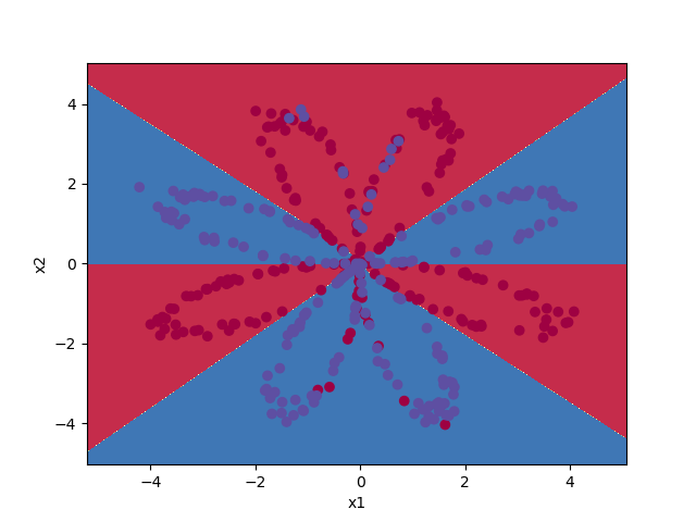
第  0  次循环,损失函数为:0.6930480201239823
第  1000  次循环,损失函数为:0.3098018601352803
第  2000  次循环,损失函数为:0.2924326333792646
第  3000  次循环,损失函数为:0.2833492852647411
第  4000  次循环,损失函数为:0.27678077562979253
第  5000  次循环,损失函数为:0.2634715508859307
第  6000  次循环,损失函数为:0.24204413129940758
第  7000  次循环,损失函数为:0.23552486626608762
第  8000  次循环,损失函数为:0.23140964509854278
第  9000  次循环,损失函数为:0.22846408048352362
准确率: 90%
作者:Ryanjie
出处:http://www.cnblogs.com/ryanjan/
本文版权归作者和博客园所有,欢迎转载。转载请在留言板处留言给我,且在文章标明原文链接,谢谢!
如果您觉得本篇博文对您有所收获,觉得我还算用心,请点击右下角的 [推荐],谢谢!

 浙公网安备 33010602011771号