Planar data classification with one hidden layer
作业简介
本次作业将实现含有一个隐藏层的神经网络,你将会体验到与之前logistic实现的不同:
- 使用含有一个隐藏层的神经网络实现2分类。
- 使用一个非线性的激活函数(比如tanh)。
- 计算交叉熵损失。
- 实现前向传播和反向传播。
工具包
sklearn包:提供简单有效的数据挖掘和数据分析。
# Package imports
import numpy as np
import matplotlib.pyplot as plt
from testCases import *
import sklearn
import sklearn.datasets
import sklearn.linear_model
from planar_utils import plot_decision_boundary, sigmoid, load_planar_dataset, load_extra_datasets

#matplotlib inline
np.random.seed(1) # set a seed so that the results are consistent
数据集
加载数据的方式:
X, Y = load_planar_dataset()
使用matplotlib可以将数据可视化:
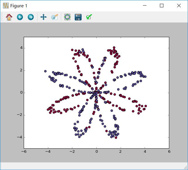
数据集类似一朵花,有红色(label y = 0)和蓝色(label y = 1)的点构成,我们的目的就是去拟合这个数据。
获取数据的维度:
shape_X = X.shape
shape_Y = Y.shape
m = shape_X[1]  # training set size
测试:
print ('The shape of X is: ' + str(shape_X))
print ('The shape of Y is: ' + str(shape_Y))
print ('I have m = %d training examples!' % (m))
输出:
The shape of X is: (2, 400)
The shape of Y is: (1, 400)
I have m = 400 training examples!
简单的逻辑回归
在建立全连接之前,我们首先来看一下逻辑回归对于该问题的表现,可以使用sklearn的内建函数来实现:
# Train the logistic regression classifier
clf = sklearn.linear_model.LogisticRegressionCV()
clf.fit(X.T, Y.T.ravel())

# Plot the decision boundary for logistic regression
plot_decision_boundary(lambda x: clf.predict(x), X, Y)
plt.title("Logistic Regression")

# Print accuracy
LR_predictions = clf.predict(X.T)
print ('Accuracy of logistic regression: %d ' % float((np.dot(Y,LR_predictions) + np.dot(1-Y,1-LR_predictions))/float(Y.size)*100) +
       '% ' + "(percentage of correctly labelled datapoints)")
plt.show()
输出: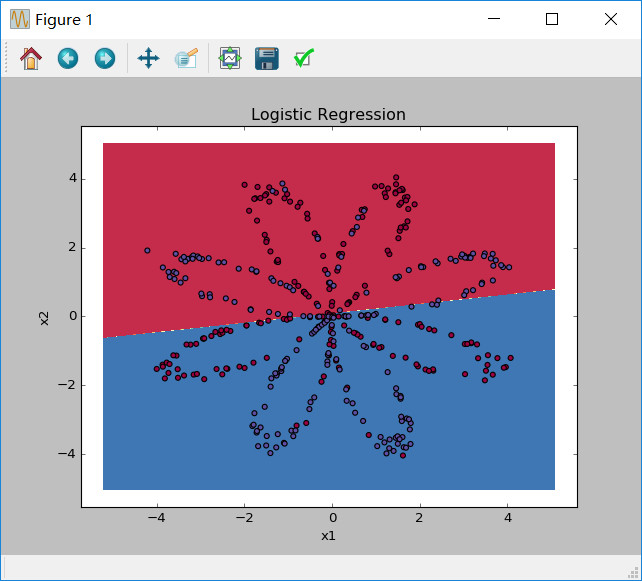
Accuracy of logistic regression: 47 % (percentage of correctly labelled datapoints)
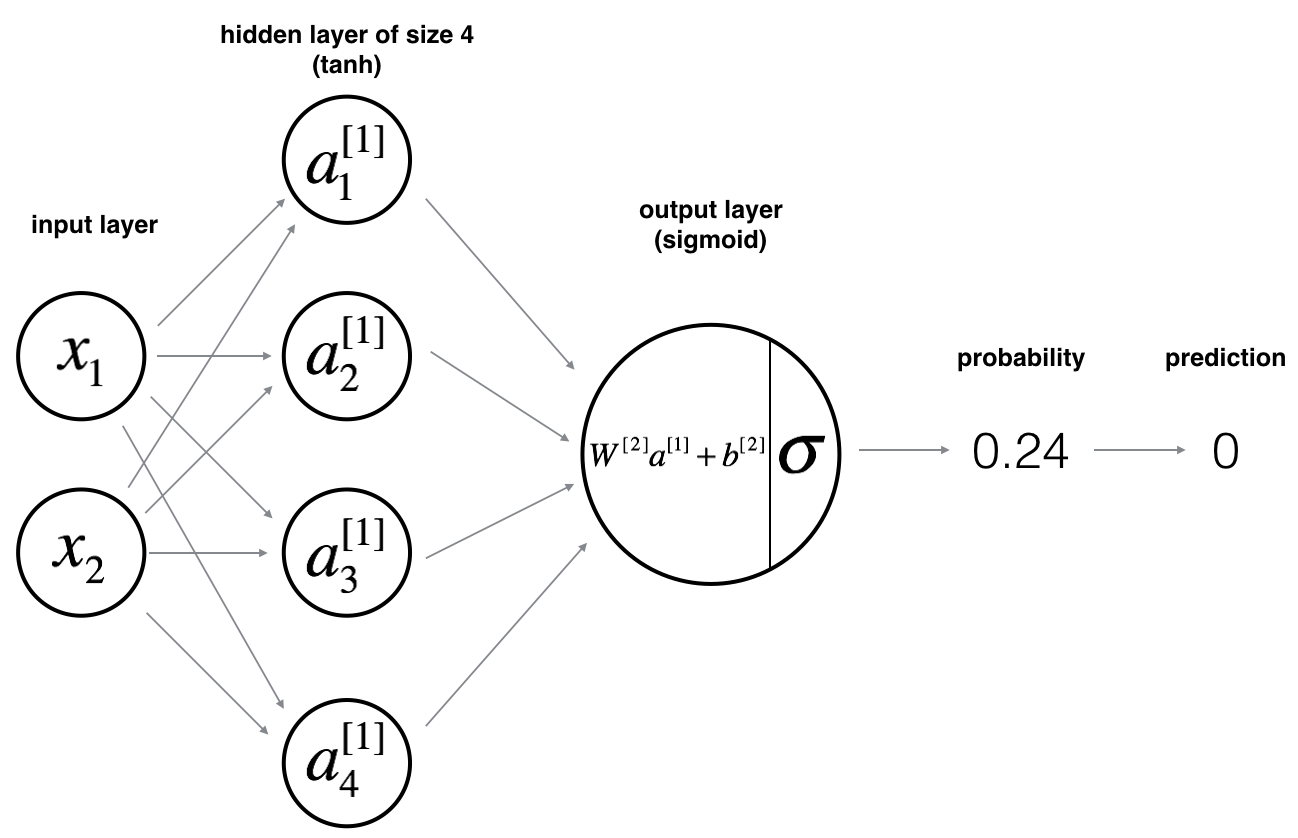
神经网络模型
由上面可以看出logistic模型对于解决“flower dataset”效果并不好,这里我们创建一个隐藏层的神经网络,下图是我们使用的网络模型:
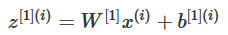
数学表达式:
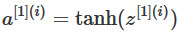
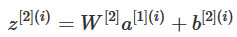
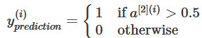
对于输入${x^{[i]}}$:

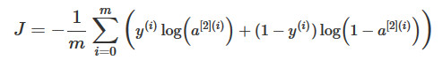
对于所有样本,损失函数J的计算:
构建神经网络的基本步骤:
- 定义神经网络的结构(输入单元,隐藏单元等)
- 初始化模型参数
- 循环
- 执行前向传播
- 计算损失
- 执行反向传播
- 更新参数(梯度下降)
通常我们将1-3步骤创建为功能函数,然后再将它们合并为一个函数,我们称为nn_model(),创建了nn_model()函数之后我们就可以进行预测。
定义神经网络结构
定义三个变量:
n_x:输入层单元数目
n_h:隐藏层单元数目
n_y:输出层单元数目
# GRADED FUNCTION: layer_sizes
def layer_sizes(X, Y):
    n_x = X.shape[0] # size of input layer
    n_h = 4
    n_y = Y.shape[0] # size of output layer
    return (n_x, n_h, n_y)
测试:
X_assess, Y_assess = layer_sizes_test_case()
(n_x, n_h, n_y) = layer_sizes(X_assess, Y_assess)
print("The size of the input layer is: n_x = " + str(n_x))
print("The size of the hidden layer is: n_h = " + str(n_h))
print("The size of the output layer is: n_y = " + str(n_y))
输出:
The size of the input layer is: n_x = 5
The size of the hidden layer is: n_h = 4
The size of the output layer is: n_y = 2
初始化模型参数
随机初始化权重参数,偏置参数初始化为0:
# GRADED FUNCTION: initialize_parameters
def initialize_parameters(n_x, n_h, n_y):
    np.random.seed(2) # we set up a seed so that your output matches ours although the initialization is random.

    ### START CODE HERE ### (≈ 4 lines of code)
    W1 = np.random.randn(n_h, n_x) * 0.01
    b1 = np.zeros((n_h, 1))
    W2 = np.random.randn(n_y, n_h) * 0.01
    b2 = np.zeros((n_y, 1))
    ### END CODE HERE ###

    assert (W1.shape == (n_h, n_x))
    assert (b1.shape == (n_h, 1))
    assert (W2.shape == (n_y, n_h))
    assert (b2.shape == (n_y, 1))

    parameters = {"W1": W1,
                  "b1": b1,
                  "W2": W2,
                  "b2": b2}
    return parameters
测试:
n_x, n_h, n_y = initialize_parameters_test_case()
parameters = initialize_parameters(n_x, n_h, n_y)
print("W1 = " + str(parameters["W1"]))
print("b1 = " + str(parameters["b1"]))
print("W2 = " + str(parameters["W2"]))
print("b2 = " + str(parameters["b2"]))
输出:
W1 = [[-0.00416758 -0.00056267]
 [-0.02136196  0.01640271]
 [-0.01793436 -0.00841747]
 [ 0.00502881 -0.01245288]]
b1 = [[ 0.]
 [ 0.]
 [ 0.]
 [ 0.]]
W2 = [[-0.01057952 -0.00909008  0.00551454  0.02292208]]
b2 = [[ 0.]]
循环
前向传播的计算,计算过程中需要进行缓存,缓存会作为方向传播的输入:
# GRADED FUNCTION: forward_propagation
def forward_propagation(X, parameters):
    W1 = parameters["W1"]
    b1 = parameters["b1"]
    W2 = parameters["W2"]
    b2 = parameters["b2"]

    # Implement Forward Propagation to calculate A2 (probabilities)
    Z1 = np.dot(W1, X) + b1
    A1 = np.tanh(Z1)
    Z2 = np.dot(W2, A1) + b2
    A2 = sigmoid(Z2)
    assert(A2.shape == (1, X.shape[1]))
    cache = {"Z1": Z1,
             "A1": A1,
             "Z2": Z2,
             "A2": A2}
    return A2, cache
测试:
X_assess, parameters = forward_propagation_test_case()
A2, cache = forward_propagation(X_assess, parameters)
# Note: we use the mean here just to make sure that your output matches ours.
print(np.mean(cache['Z1']) ,np.mean(cache['A1']),np.mean(cache['Z2']),np.mean(cache['A2']))
输出:
-0.000499755777742 -0.000496963353232 0.000438187450959 0.500109546852
交叉熵J计算:
# GRADED FUNCTION: compute_cost
def compute_cost(A2, Y, parameters):
    m = Y.shape[1] # number of example
    # Compute the cross-entropy cost
    logprobs = np.multiply(np.log(A2), Y) + np.multiply(np.log(1-A2), (1-Y))
    cost = -1/m*np.sum(logprobs)
    cost = np.squeeze(cost)     # makes sure cost is the dimension we expect.
                                # E.g., turns [[17]] into 17
    assert(isinstance(cost, float))
    return cost
在这里的计算使用np.multiply() 然后np.sum() 或者直接使用 np.dot()都可以。
测试:
A2, Y_assess, parameters = compute_cost_test_case()
print("cost = " + str(compute_cost(A2, Y_assess, parameters)))
输出:
cost = 0.692919893776
反向传播:
# GRADED FUNCTION: backward_propagation
def backward_propagation(parameters, cache, X, Y):
    m = X.shape[1]
    # First, retrieve W1 and W2 from the dictionary "parameters".
    W1 = parameters["W1"]
    W2 = parameters["W2"]
    # Retrieve also A1 and A2 from dictionary "cache".
    A1 = cache["A1"]
    A2 = cache["A2"]
    # Backward propagation: calculate dW1, db1, dW2, db2.
    dZ2 = A2 - Y    # (n_y,1)
    dW2 = 1 / m * np.dot(dZ2, A1.T)   # (n_y, 1) .* (1, n_h)
    db2 = 1 / m * np.sum(dZ2, axis=1, keepdims=True)
    dZ1 = np.dot(W2.T, dZ2) *  (1 - np.power(A1, 2))
    dW1 = 1 / m * np.dot(dZ1, X.T)
    db1 = 1 / m * np.sum(dZ1, axis=1, keepdims=True)
    grads = {"dW1": dW1,
             "db1": db1,
             "dW2": dW2,
             "db2": db2}

    return grads
测试:
parameters, cache, X_assess, Y_assess = backward_propagation_test_case()
grads = backward_propagation(parameters, cache, X_assess, Y_assess)
print ("dW1 = "+ str(grads["dW1"]))
print ("db1 = "+ str(grads["db1"]))
print ("dW2 = "+ str(grads["dW2"]))
print ("db2 = "+ str(grads["db2"]))
输出:
dW1 = [[ 0.01018708 -0.00708701]
 [ 0.00873447 -0.0060768 ]
 [-0.00530847  0.00369379]
 [-0.02206365  0.01535126]]
db1 = [[-0.00069728]
 [-0.00060606]
 [ 0.000364  ]
 [ 0.00151207]]
dW2 = [[ 0.00363613  0.03153604  0.01162914 -0.01318316]]
db2 = [[ 0.06589489]]
参数更新:
# GRADED FUNCTION: update_parameters
def update_parameters(parameters, grads, learning_rate = 1.2):
    # Retrieve each parameter from the dictionary "parameters"
    W1 = parameters["W1"]
    b1 = parameters["b1"]
    W2 = parameters["W2"]
    b2 = parameters["b2"]

    # Retrieve each gradient from the dictionary "grads"
    dW1 = grads["dW1"]
    db1 = grads["db1"]
    dW2 = grads["dW2"]
    db2 = grads["db2"]

    # Update rule for each parameter
    W1 -= learning_rate * dW1
    b1 -= learning_rate * db1
    W2 -= learning_rate * dW2
    b2 -= learning_rate * db2

    parameters = {"W1": W1,
                  "b1": b1,
                  "W2": W2,
                  "b2": b2}

    return parameters
测试:
parameters, grads = update_parameters_test_case()
parameters = update_parameters(parameters, grads)

print("W1 = " + str(parameters["W1"]))
print("b1 = " + str(parameters["b1"]))
print("W2 = " + str(parameters["W2"]))
print("b2 = " + str(parameters["b2"]))
输出:
W1 = [[-0.00643025  0.01936718]
 [-0.02410458  0.03978052]
 [-0.01653973 -0.02096177]
 [ 0.01046864 -0.05990141]]
b1 = [[ -1.02420756e-06]
 [  1.27373948e-05]
 [  8.32996807e-07]
 [ -3.20136836e-06]]
W2 = [[-0.01041081 -0.04463285  0.01758031  0.04747113]]
b2 = [[ 0.00010457]]
组合成nn_model()
# GRADED FUNCTION: nn_model
def nn_model(X, Y, n_h, num_iterations = 10000, print_cost=False):
    np.random.seed(3)
    n_x = layer_sizes(X, Y)[0]
    n_y = layer_sizes(X, Y)[2]

    # Initialize parameters, then retrieve W1, b1, W2, b2. Inputs: "n_x, n_h, n_y". Outputs = "W1, b1, W2, b2, parameters".
    parameters = initialize_parameters(n_x, n_h, n_y)
    W1 = parameters["W1"]
    b1 = parameters["b1"]
    W2 = parameters["W2"]
    b2 = parameters["b2"]
    # Loop (gradient descent)
    for i in range(0, num_iterations):
        # Forward propagation. Inputs: "X, parameters". Outputs: "A2, cache".
        A2, cache = forward_propagation(X, parameters)
        # Cost function. Inputs: "A2, Y, parameters". Outputs: "cost".
        cost = compute_cost(A2, Y, parameters)
        # Backpropagation. Inputs: "parameters, cache, X, Y". Outputs: "grads".
        grads = backward_propagation(parameters, cache, X, Y)
        # Gradient descent parameter update. Inputs: "parameters, grads". Outputs: "parameters".
        parameters = update_parameters(parameters, grads, learning_rate = 1.2)
        # Print the cost every 1000 iterations
        if print_cost and i % 1000 == 0:
            print ("Cost after iteration %i: %f" %(i, cost))

    return parameters
测试:
X_assess, Y_assess = nn_model_test_case()
parameters = nn_model(X_assess, Y_assess, 4, num_iterations=10000, print_cost=False)
print("W1 = " + str(parameters["W1"]))
print("b1 = " + str(parameters["b1"]))
print("W2 = " + str(parameters["W2"]))
print("b2 = " + str(parameters["b2"]))
输出:
W1 = [[-4.18496424  5.33205335]
 [-7.53806791  1.20753912]
 [-4.19265639  5.32636689]
 [ 7.53803581 -1.20755573]]
b1 = [[ 2.32936674]
 [ 3.80995932]
 [ 2.33014798]
 [-3.81000889]]
W2 = [[-6033.82337574 -6008.14278716 -6033.08759595  6008.07913792]]
b2 = [[-52.67940757]]
推测

# GRADED FUNCTION: predict
def predict(parameters, X):
    # Computes probabilities using forward propagation, and classifies to 0/1 using 0.5 as the threshold.
    A2, cache = forward_propagation(X, parameters)
    predictions = (A2 > 0.5)

    return predictions
测试:
parameters, X_assess = predict_test_case()
predictions = predict(parameters, X_assess)
print("predictions mean = " + str(np.mean(predictions)))
输出:
predictions mean = 0.666666666667
执行模型
# Build a model with a n_h-dimensional hidden layer
parameters = nn_model(X, Y, n_h = 4, num_iterations = 10000, print_cost=True)
# Plot the decision boundary
plot_decision_boundary(lambda x: predict(parameters, x.T), X, Y)
plt.title("Decision Boundary for hidden layer size " + str(4))
plt.show()
结果: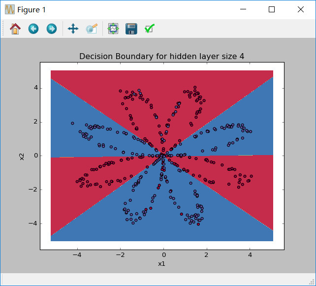
Cost after iteration 0: 0.693048
Cost after iteration 1000: 0.288083
Cost after iteration 2000: 0.254385
Cost after iteration 3000: 0.233864
Cost after iteration 4000: 0.226792
Cost after iteration 5000: 0.222644
Cost after iteration 6000: 0.219731
Cost after iteration 7000: 0.217504
Cost after iteration 8000: 0.219507
Cost after iteration 9000: 0.218621
输出准确性:
# Print accuracy
predictions = predict(parameters, X)
print ('Accuracy: %d' % float((np.dot(Y,predictions.T) + np.dot(1-Y,1-predictions.T))/float(Y.size)*100) + '%')
结果:
Accuracy: 90%
调整隐藏层大小
# This may take about 2 minutes to run
plt.figure(figsize=(16, 32))
hidden_layer_sizes = [1, 2, 3, 4, 5, 10, 20]
for i, n_h in enumerate(hidden_layer_sizes):
    plt.subplot(5, 2, i+1)
    plt.title('Hidden Layer of size %d' % n_h)
    parameters = nn_model(X, Y, n_h, num_iterations = 5000)
    plot_decision_boundary(lambda x: predict(parameters, x.T), X, Y)
    predictions = predict(parameters, X)
    accuracy = float((np.dot(Y,predictions.T) + np.dot(1-Y,1-predictions.T))/float(Y.size)*100)
    print ("Accuracy for {} hidden units: {} %".format(n_h, accuracy))
plt.show()
结果: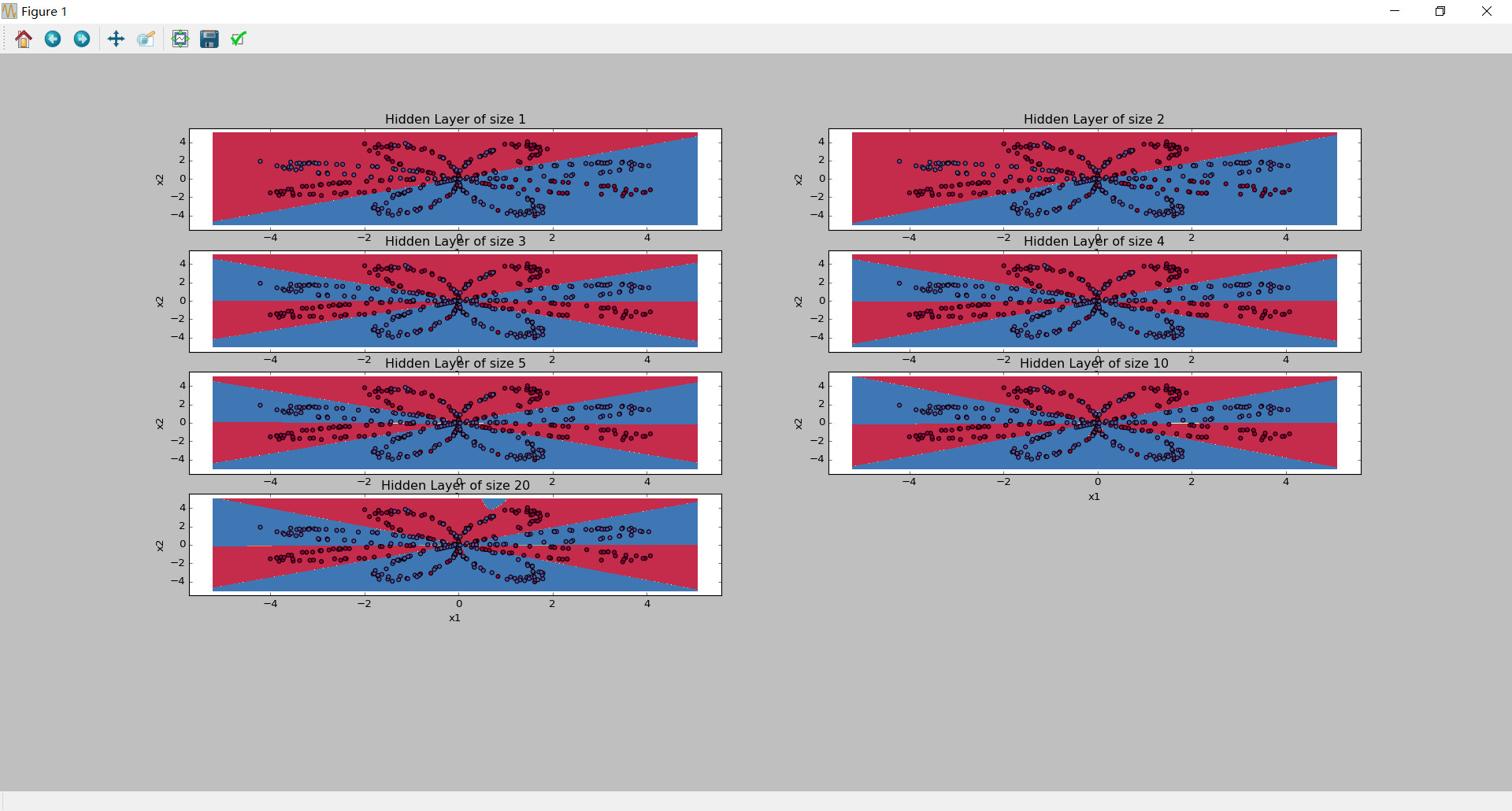
其它数据集上的表现
# Datasets
noisy_circles, noisy_moons, blobs, gaussian_quantiles, no_structure = load_extra_datasets()

datasets = {"noisy_circles": noisy_circles,
            "noisy_moons": noisy_moons,
            "blobs": blobs,
            "gaussian_quantiles": gaussian_quantiles}
dataset = "noisy_circles"
X, Y = datasets[dataset]
X, Y = X.T, Y.reshape(1, Y.shape[0])
# make blobs binary
if dataset == "noisy_moons":
    Y = Y%2
# Visualize the data
plt.scatter(X[0, :], X[1, :], c=Y, s=40, cmap=plt.cm.Spectral)
plt.show()
结果:

 浙公网安备 33010602011771号