Tensorflow-线性回归与手写数字分类

线性回归

步骤

• 构造线性回归数据
• 定义输入层
• 设计神经网络中间层
• 定义神经网络输出层
• 计算二次代价函数，构建梯度下降
• 进行训练，获取预测值
• 画图展示

代码

import tensorflow as tf
import numpy as np
import matplotlib.pyplot as plt
tf.compat.v1.disable_eager_execution()

#3-1非线性回归
#使用numpy生成200个随机点,200行1列
x_data=np.linspace(-0.5,0.5,200)[:,np.newaxis]
noise=np.random.normal(0,0.02,x_data.shape)
#square为平方
y_data=np.square(x_data)+noise
print(x_data)
print(y_data)
print(y_data.shape)

#定义两个placeholder
#输入层：一个神经元
x=tf.compat.v1.placeholder(tf.float32,[None,1])
y=tf.compat.v1.placeholder(tf.float32,[None,1])

#定义神经网络中间层
#中间层：10个神经元
Weights_L1=tf.Variable(tf.compat.v1.random_normal([1,10]))
biases_L1=tf.Variable(tf.zeros([1,10]))
Wx_plus_b_L1=tf.matmul(x,Weights_L1)+biases_L1
#L1中间层的输出，tanh为激活函数
L1=tf.nn.tanh(Wx_plus_b_L1)


#定义神经网络输出层
#输出层：一个神经元
Weights_L2=tf.Variable(tf.compat.v1.random_normal([10,1]))
biases_L2=tf.Variable(tf.zeros([1,1]))
#输出层的输入就是中间层的输出，故为L1
Wx_plus_b_L2=tf.matmul(L1,Weights_L2)+biases_L2
#预测结果
prediction=tf.nn.tanh(Wx_plus_b_L2)


#二次代价函数
#真实值减去预测值的平方的平均值
loss=tf.reduce_mean(tf.square(y-prediction))
#梯度下降：学习率，最下化为loss
train_step=tf.compat.v1.train.GradientDescentOptimizer(0.1).minimize(loss)

#定义会话
with tf.compat.v1.Session() as sess:
    # 变量初始化
    sess.run(tf.compat.v1.global_variables_initializer())
    # 开始训练
    for _ in range(2000):
        #使用placeholder进行传值，传入样本值
        sess.run(train_step,feed_dict={x:x_data,y:y_data})

    #训练好后，获得预测值，同时传入样本参数
    prediction_value=sess.run(prediction,feed_dict={x:x_data})

    #画图
    plt.figure()
    # 用散点图，来画出样本点
    plt.scatter(x_data,y_data)
    # 预测图，红色实现，线款为5
    plt.plot(x_data,prediction_value,'r-',lw=5)
    plt.show()

展示

 

 

 

手写数字分类

MNIST数据集

MNIST数据集的官网：Yann LeCun's website下载下来的数据集被分成两部分：60000行的训练数据集（mnist.train）和10000行的测试数据集（mnist.test）

数据集详情

每一张图片包含28*28个像素，我们把这一个数组展开成一个向量，长度是28*28=784。因此在
MNIST训练数据集中mnist.train.images 是一个形状为 [60000, 784] 的张量，第一个维度数字用
来索引图片，第二个维度数字用来索引每张图片中的像素点。图片里的某个像素的强度值介于0-1
之间。

 

 

 

 

 

 神经网络搭建

 

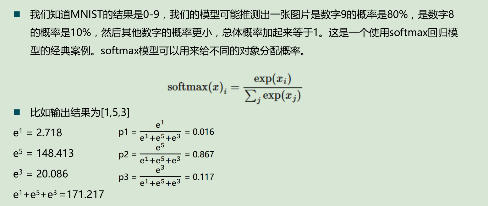
 Softmax函数

 

 代码

import tensorflow as tf
from tensorflow.examples.tutorials.mnist import input_data
tf.compat.v1.disable_eager_execution()
import numpy as np


#载入数据集
mnist=input_data.read_data_sets("MNIST_data",one_hot=True)

#每个批次大小
batch_size=100
#计算一共有多少个批次
n_bath=mnist.train.num_examples // batch_size
print(n_bath)
#定义两个placeholder
x=tf.compat.v1.placeholder(tf.float32,[None,784])
y=tf.compat.v1.placeholder(tf.float32,[None,10])

#创建一个简单的神经网络
W=tf.Variable(tf.zeros([784,10]))
b=tf.Variable(tf.zeros([10]))
prediction=tf.nn.softmax(tf.matmul(x,W)+b)


#二次代价函数
loss=tf.reduce_mean(tf.square(y-prediction))
#梯度下降
train_step=tf.compat.v1.train.GradientDescentOptimizer(0.2).minimize(loss)

#初始化变量
init=tf.compat.v1.global_variables_initializer()

#结果存放在一个布尔型列表中
#返回的是一系列的True或False argmax返回一维张量中最大的值所在的位置，对比两个最大位置是否一致
correct_prediction=tf.equal(tf.argmax(y,1),tf.argmax(prediction,1))

#求准确率
#cast：将布尔类型转换为float，将True为1.0，False为0，然后求平均值
accuracy=tf.reduce_mean(tf.cast(correct_prediction,tf.float32))


with tf.compat.v1.Session() as sess:
    sess.run(init)
    for epoch in range(21):
        for batch in range(n_bath):
            #获得一批次的数据，batch_xs为图片，batch_ys为图片标签
            batch_xs,batch_ys=mnist.train.next_batch(batch_size)
            #进行训练
            sess.run(train_step,feed_dict={x:batch_xs,y:batch_ys})
        #训练完一遍后，测试下准确率的变化

        acc=sess.run(accuracy,feed_dict={x:mnist.test.images,y:mnist.test.labels})
        print("Iter "+str(epoch)+",Testing Accuracy "+str(acc))

输出：

 

 优化代码

优化方面：

①批次个数减小到20

②权值不再为0，改为随机数，设置参数要尽可能小

③增加一个隐藏层，节点数是sqrt(n*l),其中n是输入节点数，l是输出节点数，故为89

④代价函数更换为：交叉熵

⑤梯度下降函数更换为-->动量随机梯度下降，如果上次的准确率比这次准确率还要大，则将0.2乘以0.5

代码：

import tensorflow as tf
from tensorflow.examples.tutorials.mnist import input_data
tf.compat.v1.disable_eager_execution()
import numpy as np


#载入数据集
mnist=input_data.read_data_sets("MNIST_data",one_hot=True)

#每个批次大小
batch_size=20
#计算一共有多少个批次
n_bath=mnist.train.num_examples // batch_size
print(n_bath)
#定义两个placeholder
x=tf.compat.v1.placeholder(tf.float32,[None,784])
y=tf.compat.v1.placeholder(tf.float32,[None,10])

#创建一个简单的神经网络
#1.初始化非常重要，参数要尽可能小
W=tf.Variable(tf.compat.v1.random_normal([784,89])/np.sqrt(784))
b=tf.Variable(tf.zeros([89]))
prediction=tf.nn.relu(tf.matmul(x,W)+b)

#第二层
#2.我增加了一个神经网络层，节点数是sqrt(n*l),其中n是输入节点数，l是输出节点数
W2=tf.Variable(tf.compat.v1.random_normal([89,10])/np.sqrt(89))
b2=tf.Variable(tf.zeros([10]))
#将其转换为概率值
prediction2=tf.nn.softmax(tf.matmul(prediction,W2)+b2)


#二次代价函数
# loss=tf.reduce_mean(tf.square(y-prediction2))
#交叉熵
loss = tf.reduce_mean(tf.nn.softmax_cross_entropy_with_logits(labels=y,logits=prediction2))
#动量随机梯度下降
#3.如果上次的准确率比这次准确率还要大，则将0.2乘以0.5
train_step=tf.compat.v1.train.MomentumOptimizer(0.2,0.5).minimize(loss)

#初始化变量
init=tf.compat.v1.global_variables_initializer()

#结果存放在一个布尔型列表中
#返回的是一系列的True或False argmax返回一维张量中最大的值所在的位置，对比两个最大位置是否一致
correct_prediction=tf.equal(tf.argmax(y,1),tf.argmax(prediction2,1))

#求准确率
#cast：将布尔类型转换为float，将True为1.0，False为0，然后求平均值
accuracy=tf.reduce_mean(tf.cast(correct_prediction,tf.float32))


with tf.compat.v1.Session() as sess:
    sess.run(init)
    for epoch in range(21):
        for batch in range(n_bath):
            #获得一批次的数据，batch_xs为图片，batch_ys为图片标签
            batch_xs,batch_ys=mnist.train.next_batch(batch_size)
            #进行训练
            sess.run(train_step,feed_dict={x:batch_xs,y:batch_ys})
        #训练完一遍后，测试下准确率的变化

        acc=sess.run(accuracy,feed_dict={x:mnist.test.images,y:mnist.test.labels})
        print("Iter "+str(epoch)+",Testing Accuracy "+str(acc))

输出：