数据分析报告2

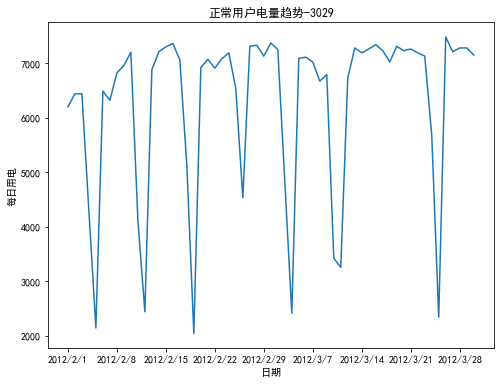
 用电预测：

import pandas as pd
import matplotlib.pyplot as plt

df_normal =pd.read_csv("C:/Users/admin/Documents/WeChat Files/wxid_b0fz4hqogenr22/FileStorage/File/2023-03/data/data/user.csv")
plt.figure(figsize=(8,6))
plt.plot(df_normal['Date'],df_normal['Eletricity'])

x_major_locator=plt.MultipleLocator(7)
ax=plt.gca()
ax.xaxis.set_major_locator(x_major_locator)
plt.rcParams['font.sans-serif']=['SimHei']

plt.ylabel('每日用电')
plt.xlabel('日期')
plt.title('正常用户电量趋势')
plt.show()

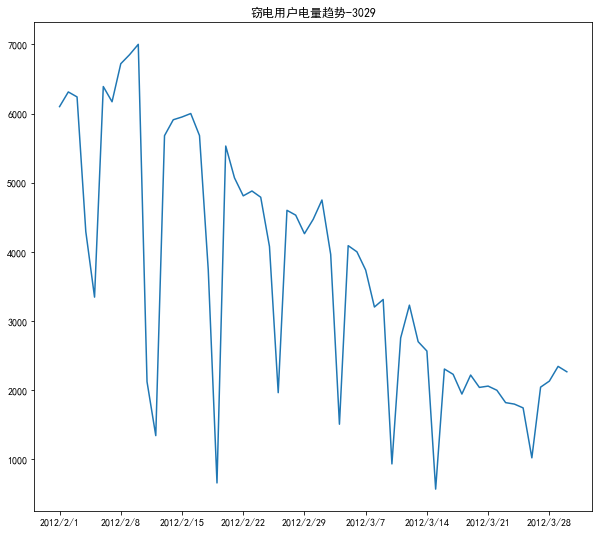
df_steal=pd.read_csv("C:/Users/admin/Documents/WeChat Files/wxid_b0fz4hqogenr22/FileStorage/File/2023-03/data/data/Steal user.csv")
plt.figure(figsize=(10,9))
plt.plot(df_steal['Date'],df_steal['Eletricity'])
'''plt.xlabel('日期')'''
'''plt.ylabel('日期')'''

x_major_locator=plt.MultipleLocator(7)
ax=plt.gca()
ax.xaxis.set_major_locator(x_major_locator)
plt.title('窃电用户电量趋势')
plt.rcParams['font.sans-serif']=['SimHei']
plt.show()

 

 

 

 

 

 

 

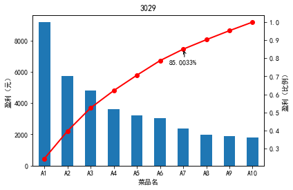
帕累托图：

import pandas as pd

dish_profit="C:/Users/admin/Documents/WeChat Files/wxid_b0fz4hqogenr22/FileStorage/File/2023-03/data/data/catering_dish_profit.xls"
data=pd.read_excel(dish_profit,index_col='菜品名')
data=data['盈利'].copy()
data.sort_values(ascending=False)

import matplotlib.pyplot as plt
plt.rcParams['font.sans-serif']=['SimHei']
plt.rcParams['axes.unicode_minus']=False
plt.figure()
data.plot(kind='bar')
plt.ylabel('盈利（元）')
p=1.0*data.cumsum()/data.sum()
p.plot(color='r',secondary_y=True,style='-o',linewidth=2)
plt.annotate(format(p[6],'.4%'),xy=(6,p[6]),xytext=(6*0.9,p[6]*0.9),arrowprops=dict(arrowstyle='->',connectionstyle='arc3,rad=.2'))
plt.ylabel('盈利（比例）')
plt.title('3029')
plt.show()

 

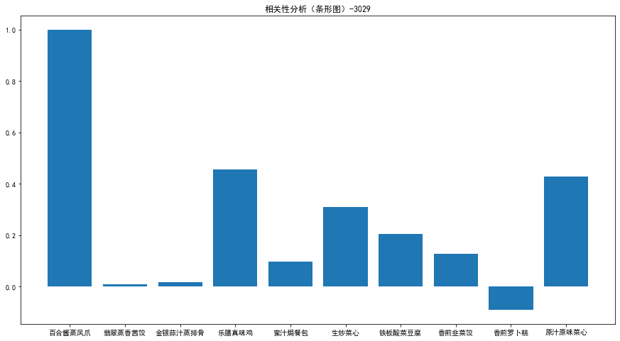
 相关性分析：

import pandas as pd
import matplotlib.pyplot as plt

catering_sale="C:/Users/admin/Documents/WeChat Files/wxid_b0fz4hqogenr22/FileStorage/File/2023-03/data/data/catering_sale_all.xls"
data=pd.read_excel(catering_sale,index_col='日期')

print(data.corr())

print(data.corr()['百合酱蒸凤爪'])

print(data['百合酱蒸凤爪'].corr(data['翡翠蒸香茜饺']))

x=['百合酱蒸凤爪', '翡翠蒸香茜饺', '金银蒜汁蒸排骨' ,'乐膳真味鸡', '蜜汁焗餐包', '生炒菜心', '铁板酸菜豆腐' ,'香煎韭菜饺', '香煎罗卜糕', '原汁原味菜心']
y=[data['百合酱蒸凤爪'].corr(data['百合酱蒸凤爪']),data['百合酱蒸凤爪'].corr(data['翡翠蒸香茜饺']),data['百合酱蒸凤爪'].corr(data['金银蒜汁蒸排骨']),data['百合酱蒸凤爪'].corr(data['乐膳真味鸡']),data['百合酱蒸凤爪'].corr(data['蜜汁焗餐包']),data['百合酱蒸凤爪'].corr(data['生炒菜心']),data['百合酱蒸凤爪'].corr(data['铁板酸菜豆腐']),data['百合酱蒸凤爪'].corr(data['香煎韭菜饺']),data['百合酱蒸凤爪'].corr(data['香煎罗卜糕']),data['百合酱蒸凤爪'].corr(data['原汁原味菜心'])]
plt.figure(figsize=(15,8))
plt.bar(x,y)
plt.rcParams['font.sans-serif']=['SimHei']

'''plt.ylabel('百合酱蒸凤爪的相关性')
plt.xlabel('菜品')'''
plt.title('相关性分析（条形图）-3029')
plt.show()

热力图：

import numpy as np
import pandas as pd
inputfile="C:/Users/admin/Documents/WeChat Files/wxid_b0fz4hqogenr22/FileStorage/File/2023-03/data.csv"
data=pd.read_csv(inputfile)
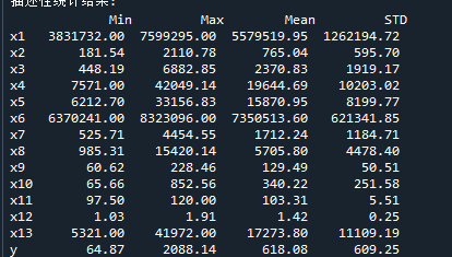
description=[data.min(),data.max(),data.mean(),data.std()]
description=pd.DataFrame(description,index=['Min','Max','Mean','STD']).T
print('描述性统计结果:\n',np.round(description,2))
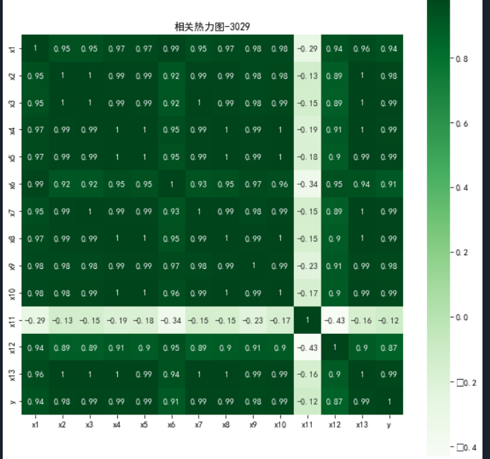
corr=data.corr(method='pearson')
import matplotlib.pyplot as plt
import seaborn as sns
plt.subplots(figsize=(10,10))
sns.heatmap(corr,annot=True,vmax=(1),square=True,cmap='Greens')
plt.title('相关热力图-3029')
plt.rcParams['font.sans-serif']=['SimHei']
plt.show()
plt.close

 

 

 Lasso回归：

import numpy as np
import pandas as pd
from sklearn.linear_model import Lasso

inputfile="C:/Users/admin/Documents/WeChat Files/wxid_b0fz4hqogenr22/FileStorage/File/2023-03/data.csv"
data=pd.read_csv(inputfile)
lasso=Lasso(1000)
lasso.fit(data.iloc[:,0:13],data['y'])
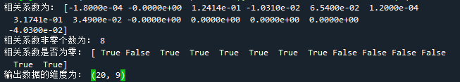
print('相关系数为：',np.round(lasso.coef_,5))

print('相关系数非零个数为：',np.sum(lasso.coef_!=0))
mask=lasso.coef_!=0
mask = np.append(mask,True)
print("相关系数是否为零：",mask)

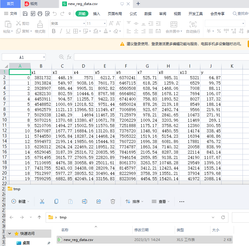
outputfile="C:/Users/admin/Desktop/tmp/new_reg_data.csv"
new_reg_data=data.iloc[:,mask]
new_reg_data.to_csv(outputfile)
print('输出数据的维度为：',new_reg_data.shape)

 

 

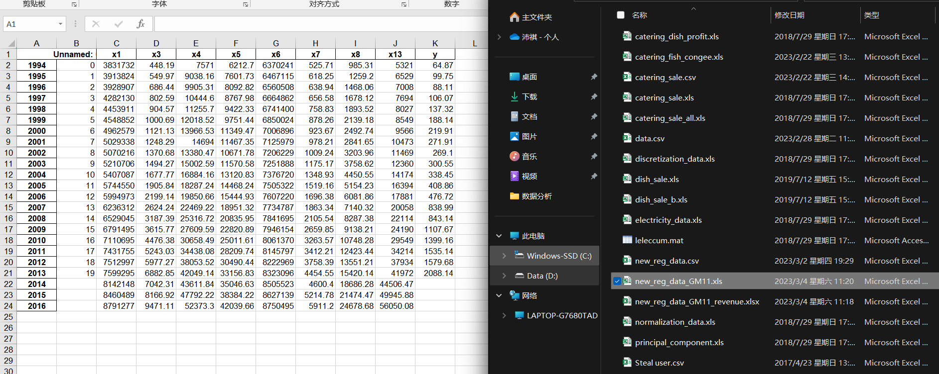
GM（1，1）灰色预测：

import sys
sys.path.append('../code') # 设置路径
import numpy as np
import pandas as pd
from GM11 import GM11 # 引入自编的灰色预测函数

inputfile1 = "D:/大三下/数据分析/data/new_reg_data.csv" # 输入的数据文件
inputfile2 = "D:/大三下/数据分析/data/data.csv"# 输入的数据文件
new_reg_data = pd.read_csv(inputfile1) # 读取经过特征选择后的数据
data = pd.read_csv(inputfile2) # 读取总的数据
new_reg_data.index = range(1994, 2014)
new_reg_data.loc[2014] = None
new_reg_data.loc[2015] = None
new_reg_data.loc[2016]=None
l = ['x1', 'x3', 'x4', 'x5', 'x6', 'x7', 'x8', 'x13']
for i in l:
f = GM11(new_reg_data.loc[range(1994, 2014),i].values)[0]
new_reg_data.loc[2014,i] = f(len(new_reg_data)-2) # 2014年预测结果
new_reg_data.loc[2015,i] = f(len(new_reg_data)-1) # 2015年预测结果
new_reg_data.loc[2016,i]=f(len(new_reg_data))
new_reg_data[i] = new_reg_data[i].round(2) # 保留两位小数
outputfile ="D:/大三下/数据分析/data/new_reg_data_GM11.xls"# 灰色预测后保存的路径
y = list(data['y'].values) # 提取财政收入列，合并至新数据框中
y.extend([np.nan,np.nan,np.nan])
new_reg_data['y'] = y
new_reg_data.to_excel(outputfile) # 结果输出
print('预测结果为：\n',new_reg_data.loc[2014:2015:2016,:]) # 预测结果展示

 

 

import matplotlib.pyplot as plt
from sklearn.svm import LinearSVR

inputfile = "C:/Users/admin/Desktop/tmp/new_reg_data_GM11.xls" # 灰色预测后保存的路径
data = pd.read_excel(inputfile,index_col=0,header=0) # 读取数据
feature = ['x1', 'x3', 'x4', 'x5', 'x6', 'x7', 'x8', 'x13'] # 属性所在列
data_train = data.loc[range(1994,2014)].copy() # 取2014年前的数据建模
data_mean = data_train.mean()
data_std = data_train.std()
data_train = (data_train - data_mean)/data_std # 数据标准化
x_train = data_train[feature].values # 属性数据
y_train = data_train['y'].values # 标签数据

linearsvr = LinearSVR() # 调用LinearSVR()函数
linearsvr.fit(x_train,y_train)
x = ((data[feature] - data_mean[feature])/data_std[feature]).values # 预测，并还原结果。
data['y_pred'] = linearsvr.predict(x) * data_std['y'] + data_mean['y']
outputfile = "C:/Users/admin/Desktop/tmp/new_reg_data_GM11_revenue.xls" # SVR预测后保存的结果
data.to_excel(outputfile)

print('真实值与预测值分别为：\n',data[['y','y_pred']])

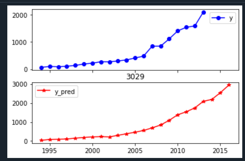
fig = data[['y','y_pred']].plot(subplots = True, style=['b-o','r-*'])
plt.title('3029') # 画出预测结果图
plt.show()