R : 山峦图

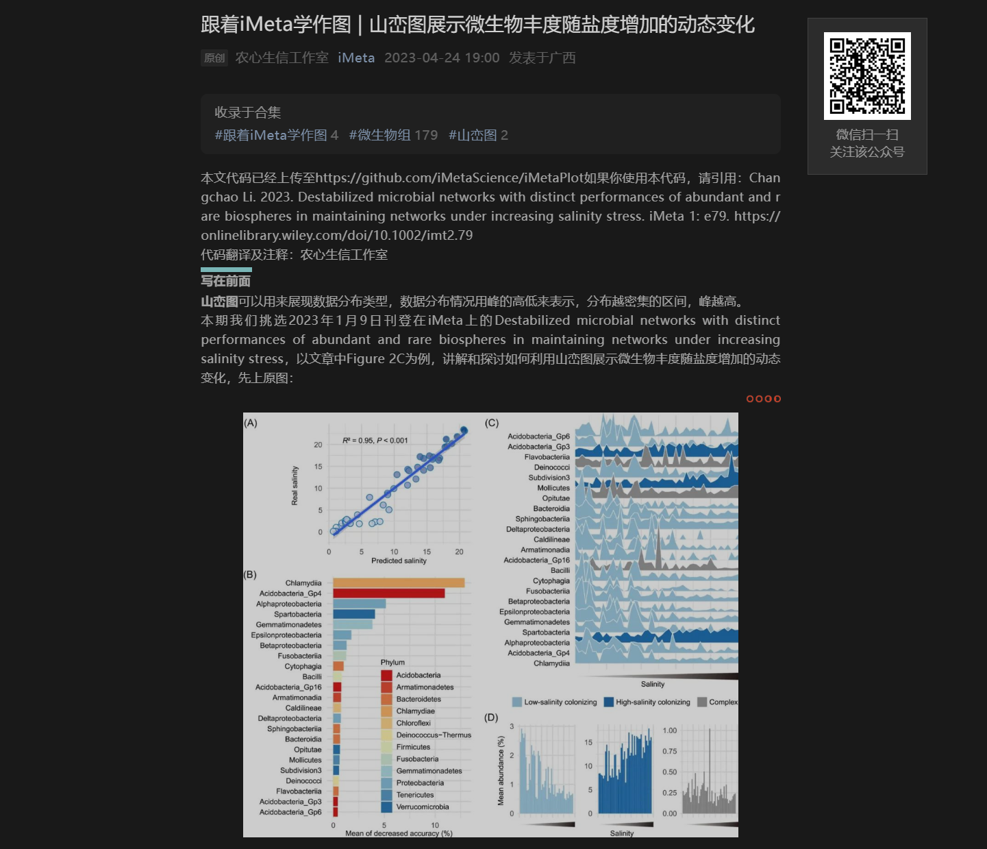
以上是学习的源头

根据课题实际做了一些修改

library(ggplot2)
library(ggridges)
library(reshape2)
library(ggsci)
setwd("C:\\Users\\Administrator\\Desktop")

otu <- read.table('feature23.txt', header = TRUE, sep = "\t")
# 对丰度标准化处理，并且转换成长数据格式
otu[2:ncol(otu)] <- scale(otu[2:ncol(otu)], center = FALSE)
otu1 <- reshape2::melt(otu, id = 'Salinity') 
# 读取分组数据
type <- read.table('feature_type.txt', header = TRUE, sep = "\t")
# 将分组数据和OTU数据合并到一起
otu2 <- merge(otu1, type, by = 'variable')

peakcol = c("#9ECAE1", "#2171B5", "#999999","#40E0D0")  
p2c <-  ggplot(otu2, aes(x = Salinity, y = variable, height = value, fill = type))+
  #主要绘制山脊线图，绘图函数里的stat参数表示对样本点做统计的方式，默认为identity，表示一个x对应一个y
  geom_ridgeline(stat = "identity", scale = 1,color = 'white', show.legend = T)+
  # 设置填充颜色，按limits（即type）填充预设的peakcol中的颜色
  scale_fill_manual(values = peakcol, limits = c('W4','W6','W8','W10'))

# 接下了需要对整体进行细节美化
p2c1 <- p2c+ 
  scale_x_continuous(breaks=c(8, 17, 26, 35), labels=c("W4", "W6", "W8", "W10"), expand = c(0, 0)) +
  theme_minimal() +
  theme(axis.title.x = element_blank(),axis.text.x.bottom = element_text()) +
  labs(x = 'Salinity ', y = 'Relative abundance of key Mo17 microbes over GrowthPeriod')
p2c1
ggsave("山峦图.pdf", p2c1, width = 8, height = 5)