

python—多视图几何
2020-04-21 22:08 工班 阅读(486) 评论(0) 收藏 举报多视图几何
一、图像之间的基础矩阵
1.1、代码实现
1.2、结果截图
1.3、小结
二、极点和极线
1.1、代码实现
1.2、结果截图
1.3 、小结
三、图像集
四、遇到的问题
五、总结
一、图像之间的基础矩阵
1.1、代码实现
  1 # -*- coding: utf-8 -*-
  2
  3 from PIL import Image
  4 from numpy import *
  5 from pylab import *
  6 import numpy as np
  7
  8 from PCV.geometry import camera
  9 from PCV.geometry import homography
 10 from PCV.geometry import sfm
 11 from PCV.localdescriptors import sift
 12
 13
 14 camera = reload(camera)
 15 homography = reload(homography)
 16 sfm = reload(sfm)
 17 sift = reload(sift)
 18
 19 # Read features
 20 im1 = array(Image.open('jia/1.jpg'))
 21 im2 = array(Image.open('jia/2.jpg'))
 22
 23
 24 sift.process_image('jia/1.jpg', 'im1.sift')
 25 l1, d1 =sift.read_features_from_file('im1.sift')
 26
 27 sift.process_image('jia/2.jpg', 'im2.sift')
 28 l2, d2 =sift.read_features_from_file('im2.sift')
 29
 30 matches = sift.match_twosided(d1, d2)
 31
 32 ndx = matches.nonzero()[0]
 33 x1 = homography.make_homog(l1[ndx, :2].T)
 34 ndx2 = [int(matches[i]) for i in ndx]
 35 x2 = homography.make_homog(l2[ndx2, :2].T)
 36
 37 d1n = d1[ndx]
 38 d2n = d2[ndx2]
 39 x1n = x1.copy()
 40 x2n = x2.copy()
 41
 42 figure(figsize=(16,16))
 43 sift.plot_matches(im1, im2, l1, l2, matches, True)
 44 show()
 45
 46 #def F_from_ransac(x1, x2, model, maxiter=5000, match_threshold=1e-6):
 47 def F_from_ransac(x1, x2, model, maxiter=5000, match_threshold=1e-6):
 48     """ Robust estimation of a fundamental matrix F from point
 49     correspondences using RANSAC (ransac.py from
 50     http://www.scipy.org/Cookbook/RANSAC).
 51
 52     input: x1, x2 (3*n arrays) points in hom. coordinates. """
 53
 54     from PCV.tools import ransac
 55     data = np.vstack((x1, x2))
 56     d = 10 # 20 is the original
 57     # compute F and return with inlier index
 58     F, ransac_data = ransac.ransac(data.T, model,
 59                                    8, maxiter, match_threshold, d, return_all=True)
 60     return F, ransac_data['inliers']
 61
 62 # find F through RANSAC
 63 model = sfm.RansacModel()
 64 F, inliers = F_from_ransac(x1n, x2n, model, maxiter=5000, match_threshold=1e-1)
 65 print("F:", F)
 66
 67 P1 = array([[1, 0, 0, 0], [0, 1, 0, 0], [0, 0, 1, 0]])
 68 P2 = sfm.compute_P_from_fundamental(F)
 69
 70 print("P2:", P2)
 71
 72 # triangulate inliers and remove points not in front of both cameras
 73 X = sfm.triangulate(x1n[:, inliers], x2n[:, inliers], P1, P2)
 74
 75 # plot the projection of X
 76 cam1 = camera.Camera(P1)
 77 cam2 = camera.Camera(P2)
 78 x1p = cam1.project(X)
 79 x2p = cam2.project(X)
 80
 81 figure(figsize=(16, 16))
 82 imj = sift.appendimages(im1, im2)
 83 imj = vstack((imj, imj))
 84
 85 imshow(imj)
 86
 87 cols1 = im1.shape[1]
 88 rows1 = im1.shape[0]
 89 for i in range(len(x1p[0])):
 90     if (0<= x1p[0][i]<cols1) and (0<= x2p[0][i]<cols1) and (0<=x1p[1][i]<rows1) and (0<=x2p[1][i]<rows1):
 91         plot([x1p[0][i], x2p[0][i]+cols1],[x1p[1][i], x2p[1][i]],'c')
 92 axis('off')
 93 show()
 94
 95 d1p = d1n[inliers]
 96 d2p = d2n[inliers]
 97
 98 # Read features
 99 im3 = array(Image.open('jia/3.jpg'))
100 sift.process_image('jia/3.jpg', 'im3.sift')
101 l3, d3 = sift.read_features_from_file('im3.sift')
102
103 matches13 = sift.match_twosided(d1p, d3)
104
105 ndx_13 = matches13.nonzero()[0]
106 x1_13 = homography.make_homog(x1p[:, ndx_13])
107 ndx2_13 = [int(matches13[i]) for i in ndx_13]
108 x3_13 = homography.make_homog(l3[ndx2_13, :2].T)
109
110 figure(figsize=(16, 16))
111 imj = sift.appendimages(im1, im3)
112 imj = vstack((imj, imj))
113
114 imshow(imj)
115
116 cols1 = im1.shape[1]
117 rows1 = im1.shape[0]
118 for i in range(len(x1_13[0])):
119     if (0<= x1_13[0][i]<cols1) and (0<= x3_13[0][i]<cols1) and (0<=x1_13[1][i]<rows1) and (0<=x3_13[1][i]<rows1):
120         plot([x1_13[0][i], x3_13[0][i]+cols1],[x1_13[1][i], x3_13[1][i]],'c')
121 axis('off')
122 show()
123
124 P3 = sfm.compute_P(x3_13, X[:, ndx_13])
125
126 print("P3:", P3)
127
128 print("P1:", P1)
129 print("P2:", P2)
130 print("P3:", P3)
调用的函数sfm.py:
  1 from pylab import *
  2 from numpy import *
  3 from scipy import linalg
  4
  5
  6 def compute_P(x,X):
  7     """    Compute camera matrix from pairs of
  8         2D-3D correspondences (in homog. coordinates). """
  9
 10     n = x.shape[1]
 11     if X.shape[1] != n:
 12         raise ValueError("Number of points don't match.")
 13
 14     # create matrix for DLT solution
 15     M = zeros((3*n,12+n))
 16     for i in range(n):
 17         M[3*i,0:4] = X[:,i]
 18         M[3*i+1,4:8] = X[:,i]
 19         M[3*i+2,8:12] = X[:,i]
 20         M[3*i:3*i+3,i+12] = -x[:,i]
 21
 22     U,S,V = linalg.svd(M)
 23
 24     return V[-1,:12].reshape((3,4))
 25
 26
 27 def triangulate_point(x1,x2,P1,P2):
 28     """ Point pair triangulation from
 29         least squares solution. """
 30
 31     M = zeros((6,6))
 32     M[:3,:4] = P1
 33     M[3:,:4] = P2
 34     M[:3,4] = -x1
 35     M[3:,5] = -x2
 36
 37     U,S,V = linalg.svd(M)
 38     X = V[-1,:4]
 39
 40     return X / X[3]
 41
 42
 43 def triangulate(x1,x2,P1,P2):
 44     """    Two-view triangulation of points in
 45         x1,x2 (3*n homog. coordinates). """
 46
 47     n = x1.shape[1]
 48     if x2.shape[1] != n:
 49         raise ValueError("Number of points don't match.")
 50
 51     X = [ triangulate_point(x1[:,i],x2[:,i],P1,P2) for i in range(n)]
 52     return array(X).T
 53
 54
 55 def compute_fundamental(x1,x2):
 56     """    Computes the fundamental matrix from corresponding points
 57         (x1,x2 3*n arrays) using the 8 point algorithm.
 58         Each row in the A matrix below is constructed as
 59         [x'*x, x'*y, x', y'*x, y'*y, y', x, y, 1] """
 60
 61     n = x1.shape[1]
 62     if x2.shape[1] != n:
 63         raise ValueError("Number of points don't match.")
 64
 65     # build matrix for equations
 66     A = zeros((n,9))
 67     for i in range(n):
 68         A[i] = [x1[0,i]*x2[0,i], x1[0,i]*x2[1,i], x1[0,i]*x2[2,i],
 69                 x1[1,i]*x2[0,i], x1[1,i]*x2[1,i], x1[1,i]*x2[2,i],
 70                 x1[2,i]*x2[0,i], x1[2,i]*x2[1,i], x1[2,i]*x2[2,i] ]
 71
 72     # compute linear least square solution
 73     U,S,V = linalg.svd(A)
 74     F = V[-1].reshape(3,3)
 75
 76     # constrain F
 77     # make rank 2 by zeroing out last singular value
 78     U,S,V = linalg.svd(F)
 79     S[2] = 0
 80     F = dot(U,dot(diag(S),V))
 81
 82     return F/F[2,2]
 83
 84
 85 def compute_epipole(F):
 86     """ Computes the (right) epipole from a
 87         fundamental matrix F.
 88         (Use with F.T for left epipole.) """
 89
 90     # return null space of F (Fx=0)
 91     U,S,V = linalg.svd(F)
 92     e = V[-1]
 93     return e/e[2]
 94
 95
 96 def plot_epipolar_line(im,F,x,epipole=None,show_epipole=True):
 97     """ Plot the epipole and epipolar line F*x=0
 98         in an image. F is the fundamental matrix
 99         and x a point in the other image."""
100
101     m,n = im.shape[:2]
102     line = dot(F,x)
103
104     # epipolar line parameter and values
105     t = linspace(0,n,100)
106     lt = array([(line[2]+line[0]*tt)/(-line[1]) for tt in t])
107
108     # take only line points inside the image
109     ndx = (lt>=0) & (lt<m)
110     plot(t[ndx],lt[ndx],linewidth=2)
111
112     if show_epipole:
113         if epipole is None:
114             epipole = compute_epipole(F)
115         plot(epipole[0]/epipole[2],epipole[1]/epipole[2],'r*')
116
117
118 def skew(a):
119     """ Skew matrix A such that a x v = Av for any v. """
120
121     return array([[0,-a[2],a[1]],[a[2],0,-a[0]],[-a[1],a[0],0]])
122
123
124 def compute_P_from_fundamental(F):
125     """    Computes the second camera matrix (assuming P1 = [I 0])
126         from a fundamental matrix. """
127
128     e = compute_epipole(F.T) # left epipole
129     Te = skew(e)
130     return vstack((dot(Te,F.T).T,e)).T
131
132
133 def compute_P_from_essential(E):
134     """    Computes the second camera matrix (assuming P1 = [I 0])
135         from an essential matrix. Output is a list of four
136         possible camera matrices. """
137
138     # make sure E is rank 2
139     U,S,V = svd(E)
140     if det(dot(U,V))<0:
141         V = -V
142     E = dot(U,dot(diag([1,1,0]),V))
143
144     # create matrices (Hartley p 258)
145     Z = skew([0,0,-1])
146     W = array([[0,-1,0],[1,0,0],[0,0,1]])
147
148     # return all four solutions
149     P2 = [vstack((dot(U,dot(W,V)).T,U[:,2])).T,
150              vstack((dot(U,dot(W,V)).T,-U[:,2])).T,
151             vstack((dot(U,dot(W.T,V)).T,U[:,2])).T,
152             vstack((dot(U,dot(W.T,V)).T,-U[:,2])).T]
153
154     return P2
155
156
157 def compute_fundamental_normalized(x1,x2):
158     """    Computes the fundamental matrix from corresponding points
159         (x1,x2 3*n arrays) using the normalized 8 point algorithm. """
160
161     n = x1.shape[1]
162     if x2.shape[1] != n:
163         raise ValueError("Number of points don't match.")
164
165     # normalize image coordinates
166     x1 = x1 / x1[2]
167     mean_1 = mean(x1[:2],axis=1)
168     S1 = sqrt(2) / std(x1[:2])
169     T1 = array([[S1,0,-S1*mean_1[0]],[0,S1,-S1*mean_1[1]],[0,0,1]])
170     x1 = dot(T1,x1)
171
172     x2 = x2 / x2[2]
173     mean_2 = mean(x2[:2],axis=1)
174     S2 = sqrt(2) / std(x2[:2])
175     T2 = array([[S2,0,-S2*mean_2[0]],[0,S2,-S2*mean_2[1]],[0,0,1]])
176     x2 = dot(T2,x2)
177
178     # compute F with the normalized coordinates
179     F = compute_fundamental(x1,x2)
180
181     # reverse normalization
182     F = dot(T1.T,dot(F,T2))
183
184     return F/F[2,2]
185
186
187 class RansacModel(object):
188     """ Class for fundmental matrix fit with ransac.py from
189         http://www.scipy.org/Cookbook/RANSAC"""
190
191     def __init__(self,debug=False):
192         self.debug = debug
193
194     def fit(self,data):
195         """ Estimate fundamental matrix using eight
196             selected correspondences. """
197
198         # transpose and split data into the two point sets
199         data = data.T
200         x1 = data[:3,:8]
201         x2 = data[3:,:8]
202
203         # estimate fundamental matrix and return
204         F = compute_fundamental_normalized(x1,x2)
205         return F
206
207     def get_error(self,data,F):
208         """ Compute x^T F x for all correspondences,
209             return error for each transformed point. """
210
211         # transpose and split data into the two point
212         data = data.T
213         x1 = data[:3]
214         x2 = data[3:]
215
216         # Sampson distance as error measure
217         Fx1 = dot(F,x1)
218         Fx2 = dot(F,x2)
219         denom = Fx1[0]**2 + Fx1[1]**2 + Fx2[0]**2 + Fx2[1]**2
220         err = ( diag(dot(x1.T,dot(F,x2))) )**2 / denom
221
222         # return error per point
223         return err
224
225
226 def F_from_ransac(x1,x2,model,maxiter=5000,match_theshold=1e-6):
227     """ Robust estimation of a fundamental matrix F from point
228         correspondences using RANSAC (ransac.py from
229         http://www.scipy.org/Cookbook/RANSAC).
230
231         input: x1,x2 (3*n arrays) points in hom. coordinates. """
232
233     from PCV.tools import ransac
234
235     data = vstack((x1,x2))
236
237     # compute F and return with inlier index
238     F,ransac_data = ransac.ransac(data.T,model,8,maxiter,match_theshold,20,return_all=True)
239     return F, ransac_data['inliers']
1.2、结果截图
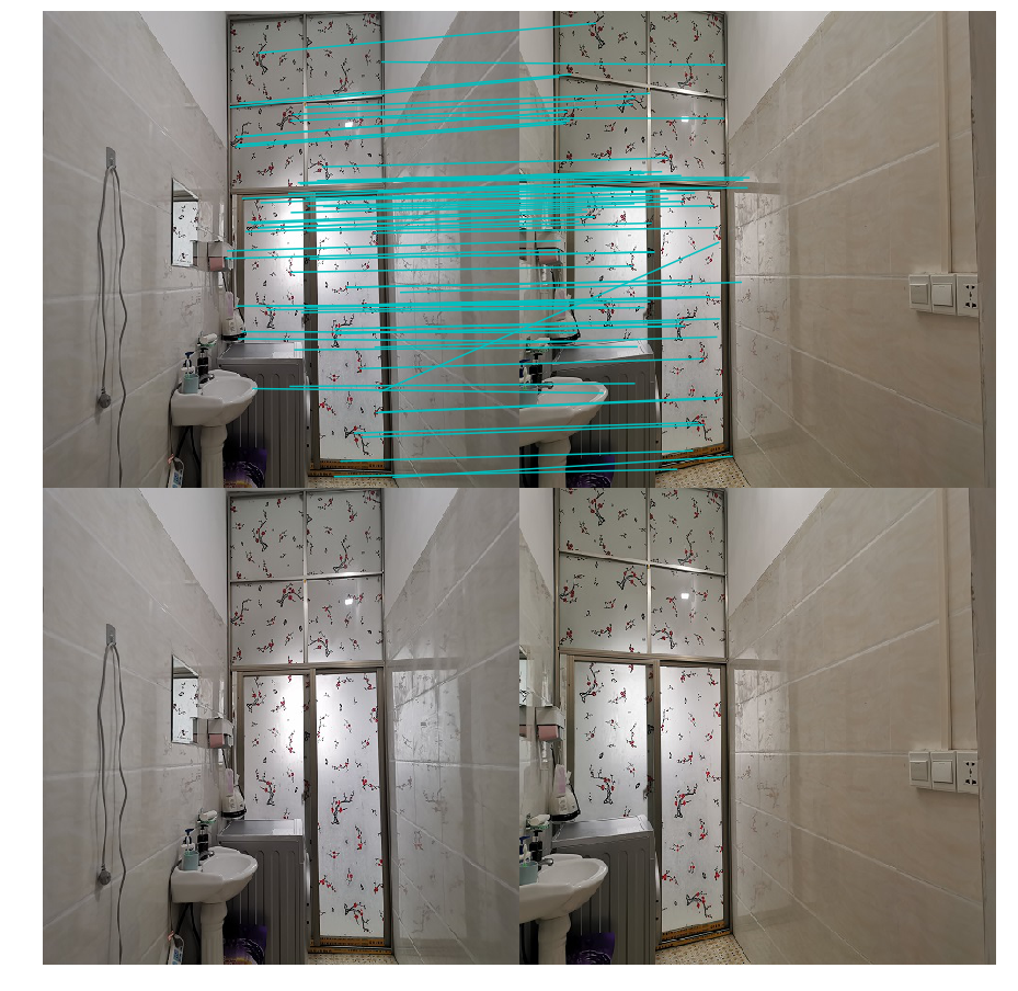
水平拍摄:
sift特征匹配:
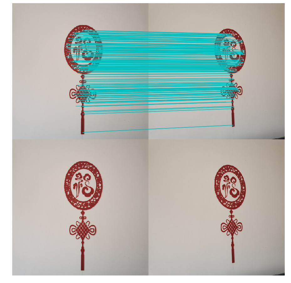
图一
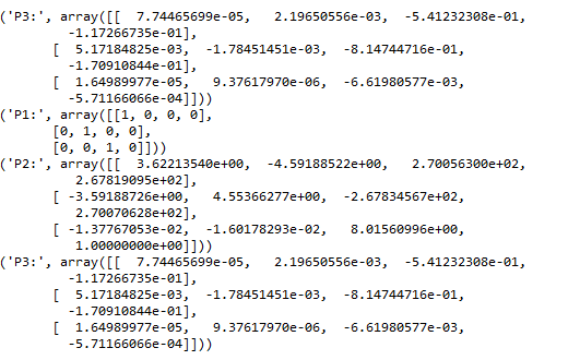
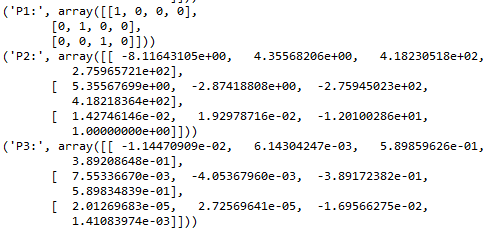
基础矩阵和投影矩阵:

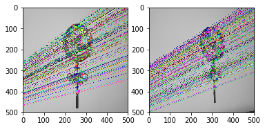
Ransac算法剔除坏的匹配点:
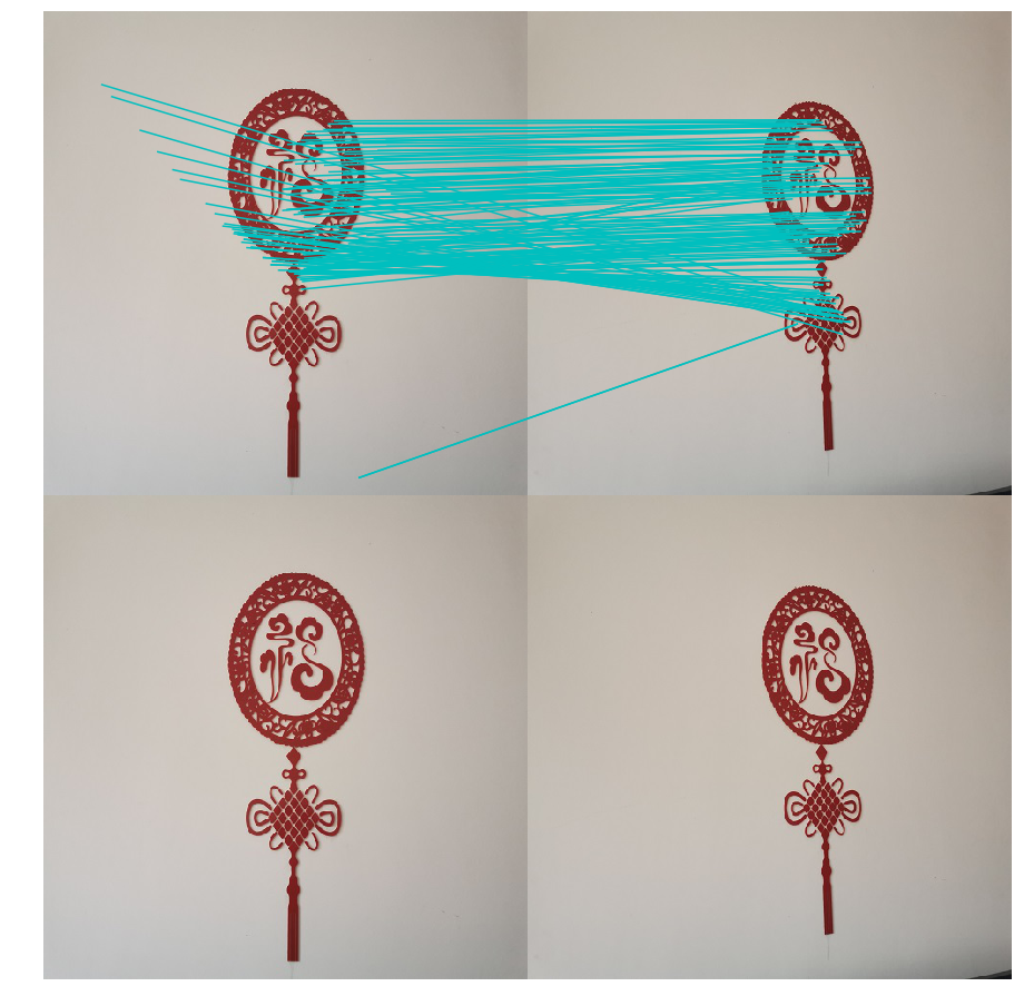
图二
8点算法匹配:
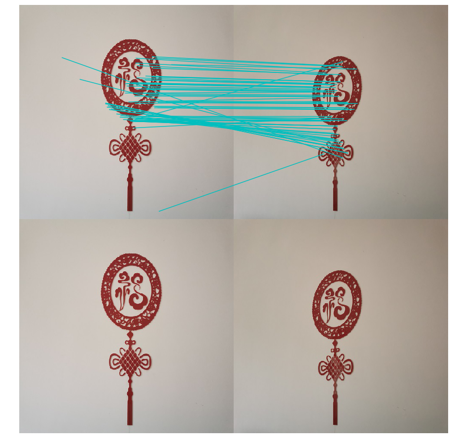
图三
左右拍摄:
sift特征匹配:
图四
基础矩阵和投影矩阵:

Ransac算法剔除坏的匹配点:

图五
8点算法匹配:

图六
基础矩阵:

前后拍摄:
sift特征匹配:
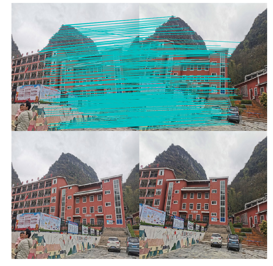
图七
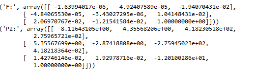
基础矩阵和投影矩阵:
Ransac算法剔除坏的匹配点:

图八
8点算法匹配:
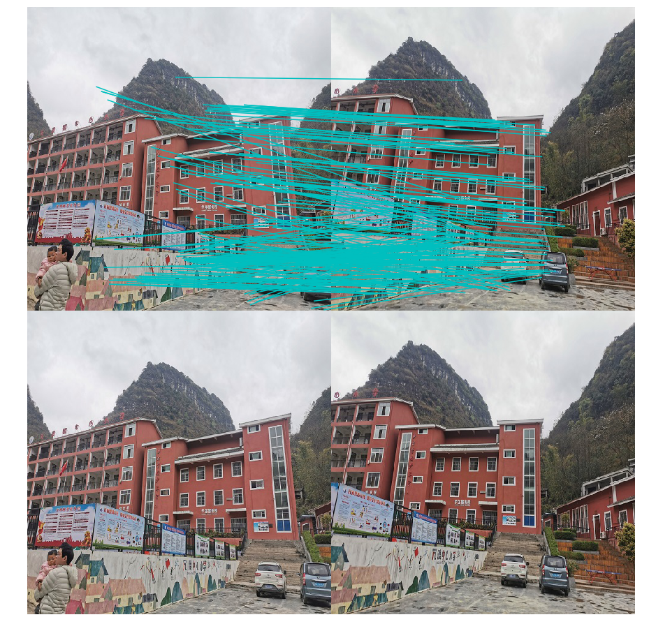
图九
两组图像的基础矩阵:
1.3、小结:提取sift特征后匹配sift特征,之后用ransac算法剔除错配的特征,然后用8点算法来求出空间中两张蹄片对应的点的坐标。
二、极点和极线
1.1、代码实现
 1 # -*- coding: utf-8 -*-
 2 import numpy as np
 3 import cv2 as cv
 4 from matplotlib import pyplot as plt
 5 img1 = cv.imread('D:/new/beizi/1.jpg',0)  #索引图像 # left image
 6 img2 = cv.imread('D:/new/beizi/2.jpg',0) #训练图像 # right image
 7 sift = cv.xfeatures2d.SIFT_create()
 8 # 使用SIFT查找关键点和描述符
 9 kp1, des1 = sift.detectAndCompute(img1,None)
10 kp2, des2 = sift.detectAndCompute(img2,None)
11 # FLANN 参数
12 FLANN_INDEX_KDTREE = 1
13 index_params = dict(algorithm = FLANN_INDEX_KDTREE, trees = 5)
14 search_params = dict(checks=50)
15 flann = cv.FlannBasedMatcher(index_params,search_params)
16 matches = flann.knnMatch(des1,des2,k=2)
17 good = []
18 pts1 = []
19 pts2 = []
20
21 for i,(m,n) in enumerate(matches):
22     if m.distance < 0.8*n.distance:
23         good.append(m)
24         pts2.append(kp2[m.trainIdx].pt)
25         pts1.append(kp1[m.queryIdx].pt)
26 pts1 = np.int32(pts1)
27 pts2 = np.int32(pts2)
28 F, mask = cv.findFundamentalMat(pts1,pts2,cv.FM_LMEDS)
29 # 我们只选择内点
30 pts1 = pts1[mask.ravel()==1]
31 pts2 = pts2[mask.ravel()==1]
32 def drawlines(img1,img2,lines,pts1,pts2):
33     ''' img1 - 我们在img2相应位置绘制极点生成的图像
34         lines - 对应的极点 '''
35     r,c = img1.shape
36     img1 = cv.cvtColor(img1,cv.COLOR_GRAY2BGR)
37     img2 = cv.cvtColor(img2,cv.COLOR_GRAY2BGR)
38     for r,pt1,pt2 in zip(lines,pts1,pts2):
39         color = tuple(np.random.randint(0,255,3).tolist())
40         x0,y0 = map(int, [0, -r[2]/r[1] ])
41         x1,y1 = map(int, [c, -(r[2]+r[0]*c)/r[1] ])
42         img1 = cv.line(img1, (x0,y0), (x1,y1), color,1)
43         img1 = cv.circle(img1,tuple(pt1),5,color,-1)
44         img2 = cv.circle(img2,tuple(pt2),5,color,-1)
45     return img1,img2
46 # 在右图(第二张图)中找到与点相对应的极点,然后在左图绘制极线
47 lines1 = cv.computeCorrespondEpilines(pts2.reshape(-1,1,2), 2,F)
48 lines1 = lines1.reshape(-1,3)
49 img5,img6 = drawlines(img1,img2,lines1,pts1,pts2)
50 # 在左图(第一张图)中找到与点相对应的Epilines,然后在正确的图像上绘制极线
51 lines2 = cv.computeCorrespondEpilines(pts1.reshape(-1,1,2), 1,F)
52 lines2 = lines2.reshape(-1,3)
53 img3,img4 = drawlines(img2,img1,lines2,pts2,pts1)
54 plt.subplot(121),plt.imshow(img5)
55 plt.subplot(122),plt.imshow(img3)
56 plt.show()
1.2、结果截图
1.3 、小结:利用SIFT查找关键点和描述符,在图中找到极点,然后用plot绘画出外极线。
三、图像集
图像集didi:
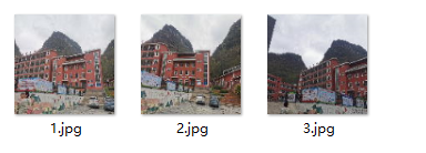
图像集jia:

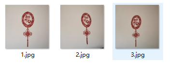
图像集beizi:
四、遇到的问题
4.1、图像的运行出现
did not meet fit acceptance criteria
持续报错,然后我就重新多拍了几组图片,换了好几组才成功的,可能是因为图像的拍摄不再一个水平和背景过于丰富。
4.2、画外极线是报错
'module' object has no attribute 'SIFT'
我找了朋友给我看了一下,跟着他改的代码就运行成功了。
五、总结
首先,图片的拍摄还是有一定的要求,我们拍摄的图片要背景不要过于丰富,尽量在一个水平线上,保持图像的清晰度,因为不清晰可能会报错或者影响实验结果,然后从三组不同的拍摄角度的图片来运行,可以看出sift匹配的点很多,室内的景使用Ransac算法剔除的坏点较多,室外的景使用的Ransac算法剔除的坏点较少,说明Ransac算法对外景的处理比较有效。从运行结果看出,外景使用8点算法匹配比较有效。求出来的基础矩阵都是三行三列,行列式值等于0(秩为2的3阶方阵),是有七个参数,其中两个参数是对级,三个参数表示两个像平面的单应性矩阵。

 浙公网安备 33010602011771号