信息论领域内的计算方法仿真，Mutual Information，互信息；

Mutual Information，互信息；

互信息，刻画的是两个变量间的相互作用；

公式如下：

要理解互信息，首先得搞懂什么是条件熵。

------

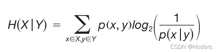
条件熵，指的是：

条件熵的基础是，条件概率。条件概率刻画的是，当时知道一件事儿时，另外一件事儿发生的概率有多大。 因此，条件熵，刻画了一个变量在给定另一个变量状态下的平均不确定性。

那么对于两个变量来说，如何量化p(x|y)呢？

------

条件熵，说的是，在给定另外一个变量时，一个变量的不确定性。（不确定性直观的理解，就是，你要搞清楚这个变量的准确状态，需要问几个“是否”问题？）

--------------

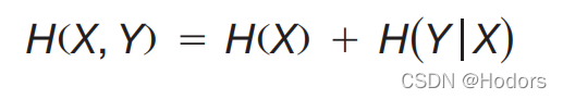
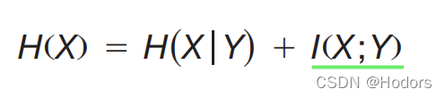
两个变量之间的不确定性，等于其中一个变量的不确定性，加上给定一个变量后，另外一个变量的不确定性。前者就是X的信息熵。后者就是已知X后，Y的条件熵。

---

那么什么是互信息呢？

第一个变量，提供了关于第二个变量的信息，这个信息量就是互信息。

mutual information。

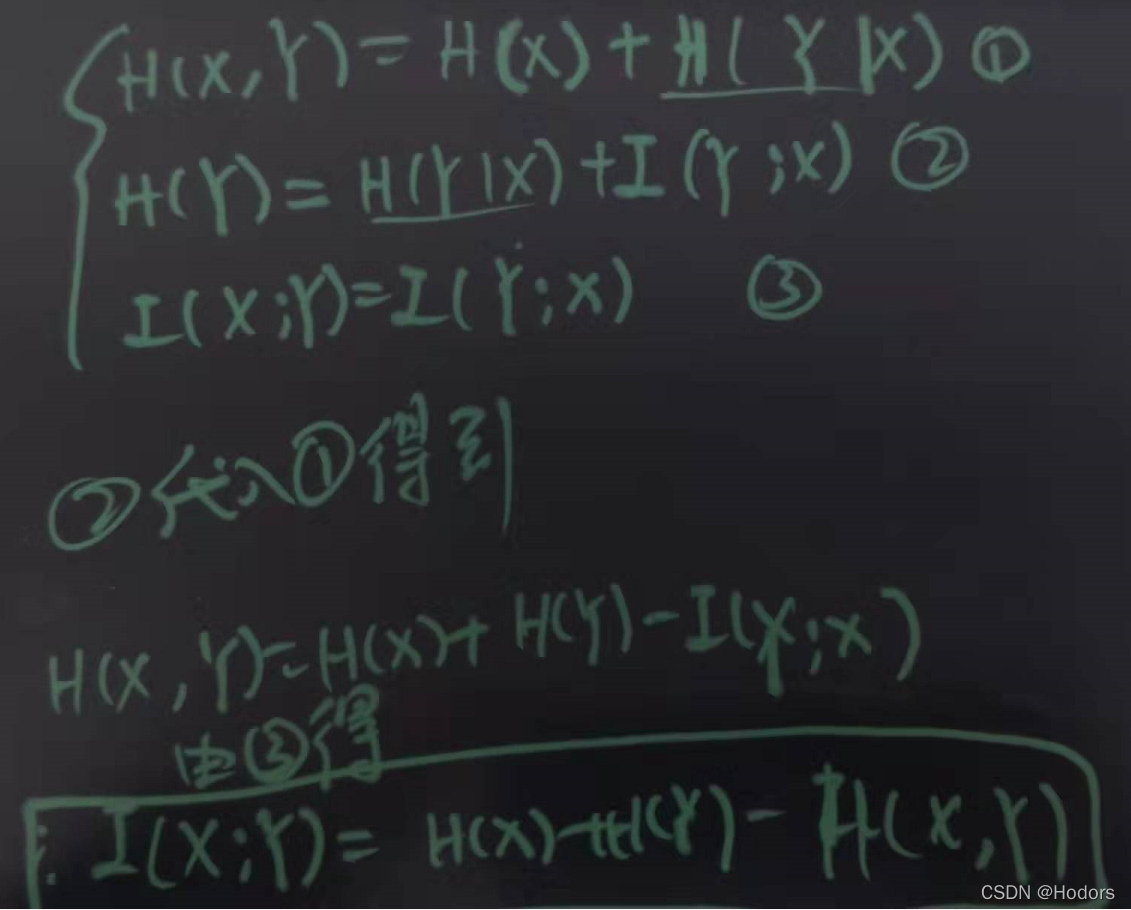
互信息的公式推导：

代码待添加。

from sklearn.metrics import mutual_info_score
import numpy as np

np.random.seed(2)

def calc_MI(x, y, bins):
    c_xy = np.histogram2d(x, y, bins)[0]
    mi = mutual_info_score(None, None, contingency=c_xy)
    return mi

x = np.random.randint(low=3, high=15, size=100, dtype=np.uint8)
y = np.random.randint(low=3, high=15, size=100, dtype=np.uint8)

mi1 = calc_MI(x, y, bins=2)
print("the MI of x,y is {:.2f}".format(mi1))
# the MI of x,y is 0.00
# 由于两个变量都是随机生成的，所以他们之间的互信息的确是0

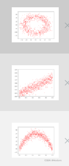
 #直线参数方程
w = 1.2
b = 0.2
x1 = np.linspace(0, 1, 1000)
noise = np.random.randn(1000)*0.2
# noise = np.random.random(1000)*0.2
y1 = w * x1 + b + noise
fig, ax = plt.subplots()
ax.scatter(x1, y1, color = 'r',s=3, label = 'add noise')
ax.set_ylim(ymin = 0, ymax = 2.0)
plt.show()


# 抛物线参数方程；
a = -8
b = 8
c = 0
x2 = np.linspace(0, 1, 1000)
noise = np.random.randn(1000)*0.3
y2 = a*x2**2 + b*x2 + c + noise
fig, ax = plt.subplots()
ax.scatter(x2, y2, color = 'r',s=3)
plt.show()

# 圆的参数方程；
r = 1.2
a, b = (0.5, 0.5)
theta = np.arange(0, 2*np.pi, 2*np.pi/1000)
x3 = a + r * np.cos(theta) + np.random.randn(1000)*0.25
y3 = b + r * np.sin(theta) + np.random.randn(1000)*0.25
fig, ax = plt.subplots()
ax.scatter(x3, y3, color = 'r',s=3)
plt.show()


#计算三者的peason相关系数；

print("case1,peason:{:.2f}".format(np.corrcoef(x1, y1)[0,1]))
print("case1,peason:{:.2f}".format(np.corrcoef(x2, y2)[0,1]))
print("case1,peason:{:.2f}".format(np.corrcoef(x3, y3)[0,1]))


#计算三者的互信息；
bin = 10
print("case1,mi:{:.2f}".format(calc_MI(x1, y1, bins=bin)))
print("case1,mi:{:.2f}".format(calc_MI(x2, y2, bins=bin)))
print("case1,mi:{:.2f}".format(calc_MI(x3, y3, bins=bin)))

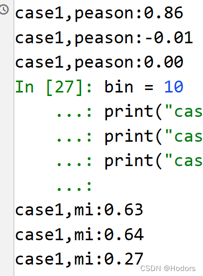
可以看到pearson只能侦测，线性关系。但是mi能够侦测到非线性关系；

--------------

如何计算两个变量的peason相关系数

Calculating Pearson Correlation Coefficient in Python with Numpy

print("case1,peason:{:.2f}".format(np.corrcoef(x1, y1)[0,1]))
print("case1,peason:{:.2f}".format(np.corrcoef(x2, y2)[0,1]))
print("case1,peason:{:.2f}".format(np.corrcoef(x3, y3)[0,1]))

---

复现figure10

 

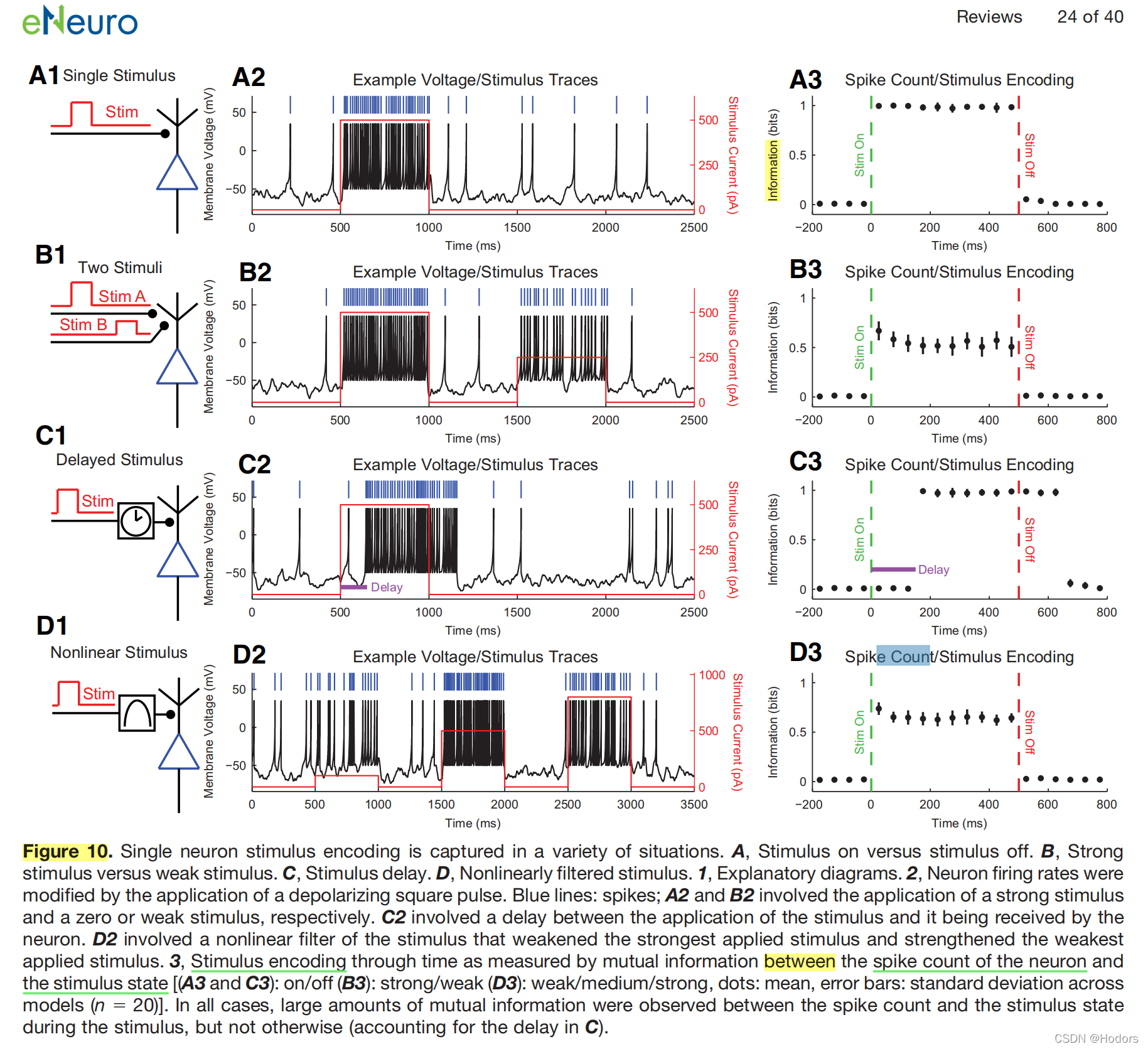
# 计算两个模态变量间的互信息，复现figure10的内容
import numpy as np

from sklearn.metrics import mutual_info_score
def calc_MI(x, y, bins):
    c_xy = np.histogram2d(x, y, bins)[0]
    mi = mutual_info_score(None, None, contingency=c_xy)
    return mi

time = range(2500)

StimulusCurrent = np.zeros(2500, dtype=int)
StimulusCurrent[500:1000] = 500
StimulusCurrent[1500:2000] = 300

MembraneVoltage = np.zeros(2500, dtype=int)
MembraneVoltage[520:1020] = 300
MembraneVoltage[1520:2020] = 150
# MembraneVoltage = MembraneVoltage + np.random.randn(2500)

bin = 10
mir = calc_MI(StimulusCurrent, MembraneVoltage, bins=bin)
print("MI result is {:.2f}".format(mir))

import matplotlib.pyplot as plt
fig, ax = plt.subplots()
ax.plot(time, StimulusCurrent, color = 'r')
ax.plot(time, MembraneVoltage, color = 'b')
ax.set_ylim(-10, 520)
plt.show()