翻译——1_Project Overview, Data Wrangling and Exploratory Analysis-checkpoint
为提高提高大学能源效率进行建筑能源需求预测
本文翻译哈佛大学的能源分析和预测报告,这是原文
暂无数据源,个人认为学习分析方法就足够
内容:
- 项目概述
- 了解数据
- 探索性分析
- 使用不同的机器学习方法进行预测
- 总结
- 结论
- 讨论
1. 项目概述
用机器学习来进行能源预测,希望能够节约能源
2. 了解数据
有三种类型的能源消耗,电力,冷水和热水。图显示了哈佛工厂供应的冷水和热水的建筑物。
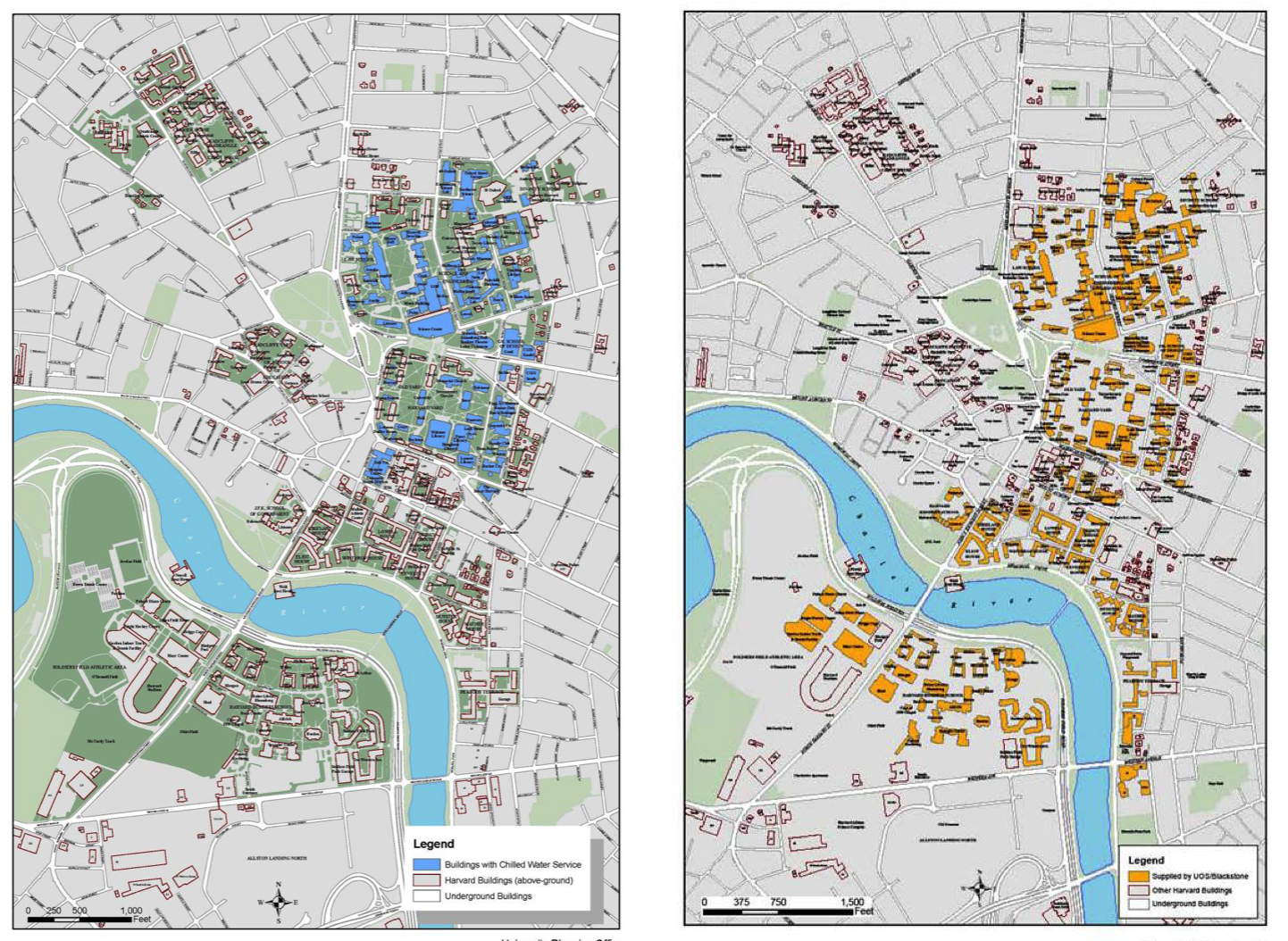
图:哈佛的冷水和热水供应。(左:冷水,用蓝色标出。右边:热水,用黄色突出显示。)
我们选择了一栋建筑,并获得了2011年7月1日至2014年10月31日的能耗数据。由于仪表故障,有几个月的数据丢失。数据分辨率是每小时一次。在原始数据中,每小时的数据是仪表读数。为了得到每小时的消耗,我们需要抵消数据然后减去。我们有2012年1月到2014年10月的每小时天气和能源数据(2.75年)。天气数据来自剑桥气象站。
在本节中,我们将完成以下任务。
。手动从哈佛能源见证网站下载原始数据,获取每小时的电力、冷水和热水。
。干净的天气数据,增加了更多的功能,包括冷度,热度和湿度比。
。根据假期、学年和周末估算每日入住率。
。创建与小时相关的特性,即cos(hourOfDay * 2 * pi / 24)。
。合并电力、冷水和热水数据流与天气、时间和占用功能。
%matplotlib inline

import requests
from StringIO import StringIO
import numpy as np
import pandas as pd # pandas
import matplotlib.pyplot as plt # module for plotting
import datetime as dt # module for manipulating dates and times
import numpy.linalg as lin # 执行线性代数运算的模块
from __future__ import division
from math import log10,exp

pd.options.display.mpl_style = 'default'
原始能耗数据
原始数据从哈佛能源见证网站下载

然后我们用Pandas 把它们放在一个dataframe里。
file = 'Data/Org/0701-0930-2011.xls'
df = pd.read_excel(file, header = 0, skiprows = np.arange(0,6))

files = ['Data/Org/1101-1130-2011.xls',
         'Data/Org/1201-2011-0131-2012.xls',
         'Data/Org/0201-0331-2012.xls',
         'Data/Org/0401-0531-2012.xls',
         'Data/Org/0101-0228-2013.xls',
         'Data/Org/0301-0430-2013.xls',
         'Data/Org/0501-0630-2013.xls',
         'Data/Org/0701-0831-2013.xls',
         'Data/Org/0901-1031-2013.xls',
         'Data/Org/1101-1231-2013.xls',
         'Data/Org/0101-0228-2014.xls',
         'Data/Org/0301-0430-2014.xls',
         'Data/Org/0501-0630-2014.xls',
         'Data/Org/0701-0831-2014.xls',
         'Data/Org/0901-1031-2014.xls']

for file in files:
    data = pd.read_excel(file, header = 0, skiprows = np.arange(0,6))
    df = df.append(data)

df.head()
WARNING *** file size (2481102) not 512 + multiple of sector size (512)
WARNING *** file size (848833) not 512 + multiple of sector size (512)
WARNING *** file size (1694257) not 512 + multiple of sector size (512)
WARNING *** file size (1640459) not 512 + multiple of sector size (512)
WARNING *** file size (1667907) not 512 + multiple of sector size (512)
WARNING *** file size (847258) not 512 + multiple of sector size (512)
WARNING *** file size (1691449) not 512 + multiple of sector size (512)
WARNING *** file size (1666647) not 512 + multiple of sector size (512)
WARNING *** file size (1665736) not 512 + multiple of sector size (512)
WARNING *** file size (1614814) not 512 + multiple of sector size (512)
WARNING *** file size (1665980) not 512 + multiple of sector size (512)
WARNING *** file size (1667276) not 512 + multiple of sector size (512)
WARNING *** file size (1691736) not 512 + multiple of sector size (512)
WARNING *** file size (1666704) not 512 + multiple of sector size (512)
WARNING *** file size (1665920) not 512 + multiple of sector size (512)
WARNING *** file size (1614900) not 512 + multiple of sector size (512)
WARNING *** file size (1666228) not 512 + multiple of sector size (512)
WARNING *** file size (1666191) not 512 + multiple of sector size (512)
WARNING *** file size (1691845) not 512 + multiple of sector size (512)
WARNING *** file size (1663846) not 512 + multiple of sector size (512)
| Unnamed: 0 | Unnamed: 1 | Gund Bus-A 15 Min Block Demand - kW | Gund Bus-A CurrentA - Amps | Unnamed: 4 | Unnamed: 5 | Gund Bus-A CurrentB - Amps | Unnamed: 7 | Gund Bus-A CurrentC - Amps | Unnamed: 9 | ... | Gund Main Demand - Tons | Gund Main Energy - Ton-Days | Gund Main FlowRate - gpm | Gund Main FlowTotal - kgal(1000) | Gund Main SignalAeration - Count | Gund Main SignalStrength - Count | Gund Main SonicVelocity - Ft/Sec | Gund Main TempDelta - Deg F | Gund Main TempReturn - Deg F | Gund Main TempSupply - Deg F | |
|---|---|---|---|---|---|---|---|---|---|---|---|---|---|---|---|---|---|---|---|---|---|
| 0 | 2011-07-01 01:00:00 | White | 48.458733 | 65.977882 | NaN | NaN | 52.631417 | NaN | 55.603840 | NaN | ... | 4.677294 | 17912.537804 | 6.916454 | 48168.083414 | 0.693405 | 57.208127 | 1437.640543 | 16.238684 | 59.757447 | 43.516103 |
| 1 | 2011-07-01 02:00:00 | White | 40.472697 | 57.230223 | NaN | NaN | 42.483092 | NaN | 50.243230 | NaN | ... | 4.586403 | 17912.853518 | 6.739337 | 48168.645429 | 0.567355 | 57.082909 | 1438.030719 | 16.263573 | 59.710199 | 43.495128 |
| 2 | 2011-07-01 03:00:00 | #d2e4b0 | 39.472809 | 55.487443 | NaN | NaN | 41.911784 | NaN | 48.482163 | NaN | ... | 4.462877 | 17913.169232 | 6.725142 | 48169.207444 | 0.441304 | 57.001646 | 1439.111130 | 15.797043 | 59.248158 | 43.457344 |
| 3 | 2011-07-01 04:00:00 | White | 39.198879 | 55.849806 | NaN | NaN | 41.525529 | NaN | 48.987457 | NaN | ... | 4.696993 | 17913.484946 | 7.041330 | 48169.769458 | 0.315254 | 57.000000 | 1440.768604 | 15.947392 | 59.207097 | 43.267682 |
| 4 | 2011-07-01 05:00:00 | White | 39.297522 | 55.736219 | NaN | NaN | 41.299381 | NaN | 48.710408 | NaN | ... | 4.550372 | 17913.800660 | 6.863004 | 48170.331473 | 0.189204 | 57.000000 | 1442.426077 | 15.903679 | 59.282707 | 43.372615 |
5 rows × 55 columns
以上是原始的每小时数据。
正如你所看到的,它很乱。首先要删除没有意义的列。
df.rename(columns={'Unnamed: 0':'Datetime'}, inplace=True)
nonBlankColumns = ['Unnamed' not in s for s in df.columns]
columns = df.columns[nonBlankColumns]
df = df[columns]
df = df.set_index(['Datetime'])
df.index.name = None
df.head()
| Gund Bus-A 15 Min Block Demand - kW | Gund Bus-A CurrentA - Amps | Gund Bus-A CurrentB - Amps | Gund Bus-A CurrentC - Amps | Gund Bus-A CurrentN - Amps | Gund Bus-A EnergyReal - kWhr | Gund Bus-A Freq - Hertz | Gund Bus-A Max Monthly Demand - kW | Gund Bus-A PowerApp - kVA | Gund Bus-A PowerReac - kVAR | ... | Gund Main Demand - Tons | Gund Main Energy - Ton-Days | Gund Main FlowRate - gpm | Gund Main FlowTotal - kgal(1000) | Gund Main SignalAeration - Count | Gund Main SignalStrength - Count | Gund Main SonicVelocity - Ft/Sec | Gund Main TempDelta - Deg F | Gund Main TempReturn - Deg F | Gund Main TempSupply - Deg F | |
|---|---|---|---|---|---|---|---|---|---|---|---|---|---|---|---|---|---|---|---|---|---|
| 2011-07-01 01:00:00 | 48.458733 | 65.977882 | 52.631417 | 55.603840 | 15.982278 | 1796757.502803 | 59.837524 | 96.117915 | 48.757073 | 12.344712 | ... | 4.677294 | 17912.537804 | 6.916454 | 48168.083414 | 0.693405 | 57.208127 | 1437.640543 | 16.238684 | 59.757447 | 43.516103 |
| 2011-07-01 02:00:00 | 40.472697 | 57.230223 | 42.483092 | 50.243230 | 13.423762 | 1796800.145991 | 60.005569 | 96.117915 | 42.238685 | 12.967984 | ... | 4.586403 | 17912.853518 | 6.739337 | 48168.645429 | 0.567355 | 57.082909 | 1438.030719 | 16.263573 | 59.710199 | 43.495128 |
| 2011-07-01 03:00:00 | 39.472809 | 55.487443 | 41.911784 | 48.482163 | 13.478933 | 1796840.146023 | 59.833880 | 96.117915 | 41.278573 | 12.732046 | ... | 4.462877 | 17913.169232 | 6.725142 | 48169.207444 | 0.441304 | 57.001646 | 1439.111130 | 15.797043 | 59.248158 | 43.457344 |
| 2011-07-01 04:00:00 | 39.198879 | 55.849806 | 41.525529 | 48.987457 | 13.603309 | 1796879.023607 | 59.673044 | 96.117915 | 41.345776 | 12.687845 | ... | 4.696993 | 17913.484946 | 7.041330 | 48169.769458 | 0.315254 | 57.000000 | 1440.768604 | 15.947392 | 59.207097 | 43.267682 |
| 2011-07-01 05:00:00 | 39.297522 | 55.736219 | 41.299381 | 48.710408 | 13.797331 | 1796918.273558 | 59.986672 | 96.117915 | 41.166736 | 12.437842 | ... | 4.550372 | 17913.800660 | 6.863004 | 48170.331473 | 0.189204 | 57.000000 | 1442.426077 | 15.903679 | 59.282707 | 43.372615 |
5 rows × 48 columns
然后我们打印出所有的列名。只有几根柱子可用来获得每小时的电力、冷水和热水。
for item in df.columns:
    print item
Gund Bus-A 15 Min Block Demand - kW
Gund Bus-A CurrentA - Amps
Gund Bus-A CurrentB - Amps
Gund Bus-A CurrentC - Amps
Gund Bus-A CurrentN - Amps
Gund Bus-A EnergyReal - kWhr
Gund Bus-A Freq - Hertz
Gund Bus-A Max Monthly Demand - kW
Gund Bus-A PowerApp - kVA
Gund Bus-A PowerReac - kVAR
Gund Bus-A PowerReal - kW
Gund Bus-A TruePF - PF
Gund Bus-A VoltageAB - Volts
Gund Bus-A VoltageAN - Volts
Gund Bus-A VoltageBC - Volts
Gund Bus-A VoltageBN - Volts
Gund Bus-A VoltageCA - Volts
Gund Bus-A VoltageCN - Volts
Gund Bus-B 15 Min Block Demand - kW
Gund Bus-B CurrentA - Amps
Gund Bus-B CurrentB - Amps
Gund Bus-B CurrentC - Amps
Gund Bus-B CurrentN - Amps
Gund Bus-B EnergyReal - kWhr
Gund Bus-B Freq - Hertz
Gund Bus-B Max Monthly Demand - kW
Gund Bus-B PowerApp - kVA
Gund Bus-B PowerReac - kVAR
Gund Bus-B PowerReal - kW
Gund Bus-B TruePF - PF
Gund Bus-B VoltageAB - Volts
Gund Bus-B VoltageAN - Volts
Gund Bus-B VoltageBC - Volts
Gund Bus-B VoltageBN - Volts
Gund Bus-B VoltageCA - Volts
Gund Bus-B VoltageCN - Volts
Gund Condensate Counter - count
Gund Condensate FlowTotal - LBS
Gund Main Demand - Tons
Gund Main Energy - Ton-Days
Gund Main FlowRate - gpm
Gund Main FlowTotal - kgal(1000)
Gund Main SignalAeration - Count
Gund Main SignalStrength - Count
Gund Main SonicVelocity - Ft/Sec
Gund Main TempDelta - Deg F
Gund Main TempReturn - Deg F
Gund Main TempSupply - Deg F
电力
以电力为例,“Gund Bus A”和“Gund Bus B”。“EnergyReal - kWhr”记录累计消耗量。我们不确定什么是“PowerReal”。为了以防万一,我们也把它放进了电日计。
electricity=df[['Gund Bus-A EnergyReal - kWhr',
                'Gund Bus-B EnergyReal - kWhr',
                'Gund Bus-A PowerReal - kW',
                'Gund Bus-B PowerReal - kW',]]
electricity.head()
| Gund Bus-A EnergyReal - kWhr | Gund Bus-B EnergyReal - kWhr | Gund Bus-A PowerReal - kW | Gund Bus-B PowerReal - kW | |
|---|---|---|---|---|
| 2011-07-01 01:00:00 | 1796757.502803 | 3657811.582122 | 47.184015 | 63.486186 |
| 2011-07-01 02:00:00 | 1796800.145991 | 3657873.464938 | 40.208796 | 61.270542 |
| 2011-07-01 03:00:00 | 1796840.146023 | 3657934.837505 | 39.209866 | 61.464394 |
| 2011-07-01 04:00:00 | 1796879.023607 | 3657995.470348 | 39.378507 | 59.396581 |
| 2011-07-01 05:00:00 | 1796918.273558 | 3658054.470285 | 39.240837 | 58.911729 |
通过检查每月的能耗来验证我们的数据处理方法
为了检验我们对数据的理解是否正确,我们想从每小时的数据中计算出每个月的用电量,然后将结果与facalities提供的每个月的数据进行比较,这些数据也可以在Energy Witness上找到。
以下是facalities提供的月度数据,"Bus A & B"以月度形式称为"CE603B kWh"和"CE604B kWh"。请注意,查表周期不是公历月份。
file = 'Data/monthly electricity.csv'
monthlyElectricityFromFacility = pd.read_csv(file, header=0)
monthlyElectricityFromFacility
monthlyElectricityFromFacility = monthlyElectricityFromFacility.set_index(['month'])
monthlyElectricityFromFacility.head()
| startDate | endDate | CE603B kWh | CE604B kWh | |
|---|---|---|---|---|
| month | ||||
| Jul 11 | 6/16/11 | 7/18/11 | 43968.1 | 106307.1 |
| Aug 11 | 7/18/11 | 8/17/11 | 41270.1 | 83121.1 |
| Sep 11 | 8/17/11 | 9/16/11 | 51514.1 | 107083.1 |
| Oct 11 | 9/16/11 | 10/18/11 | 65338.1 | 114350.1 |
| Nov 11 | 10/18/11 | 11/17/11 | 65453.1 | 115318.1 |
我们用“EnergyReal - kWhr”列表示两个电表。我们计算了查表周期的开始日期和结束日期的数字,用结束日期的数字减去开始日期的数字,就得到了每月的电量消耗。
monthlyElectricityFromFacility['startDate'] = pd.to_datetime(monthlyElectricityFromFacility['startDate'], format="%m/%d/%y")
values = monthlyElectricityFromFacility.index.values

keys = np.array(monthlyElectricityFromFacility['startDate'])

dates = {}
for key, value in zip(keys, values):
    dates[key] = value

sortedDates =  np.sort(dates.keys())
sortedDates = sortedDates[sortedDates > np.datetime64('2011-11-01')]

months = []
monthlyElectricityOrg = np.zeros((len(sortedDates) - 1, 2))
for i in range(len(sortedDates) - 1):
    begin = sortedDates[i]
    end = sortedDates[i+1]
    months.append(dates[sortedDates[i]])
    monthlyElectricityOrg[i, 0] = (np.round(electricity.loc[end,'Gund Bus-A EnergyReal - kWhr']
                           -  electricity.loc[begin,'Gund Bus-A EnergyReal - kWhr'], 1))
    monthlyElectricityOrg[i, 1] = (np.round(electricity.loc[end,'Gund Bus-B EnergyReal - kWhr']
                           -  electricity.loc[begin,'Gund Bus-B EnergyReal - kWhr'], 1))

monthlyElectricity = pd.DataFrame(data = monthlyElectricityOrg, index = months, columns = ['CE603B kWh', 'CE604B kWh'])


plt.figure()
fig, ax = plt.subplots()
fig = monthlyElectricity.plot(marker = 'o', figsize=(15,6), rot = 40, fontsize = 13, ax = ax, linestyle='')
fig.set_axis_bgcolor('w')
plt.xlabel('Billing month', fontsize = 15)
plt.ylabel('kWh', fontsize = 15)
plt.tick_params(which=u'major', reset=False, axis = 'y', labelsize = 13)
plt.xticks(np.arange(0,len(months)),months)
plt.title('Original monthly consumption from hourly data',fontsize = 17)

text = 'Meter malfunction'
ax.annotate(text, xy = (9, 4500000),
            xytext = (5, 2), fontsize = 15,
            textcoords = 'offset points', ha = 'center', va = 'top')

ax.annotate(text, xy = (8, -4500000),
            xytext = (5, 2), fontsize = 15,
            textcoords = 'offset points', ha = 'center', va = 'bottom')

ax.annotate(text, xy = (14, -2500000),
            xytext = (5, 2), fontsize = 15,
            textcoords = 'offset points', ha = 'center', va = 'bottom')

ax.annotate(text, xy = (15, 2500000),
            xytext = (5, 2), fontsize = 15,
            textcoords = 'offset points', ha = 'center', va = 'top')

plt.show()
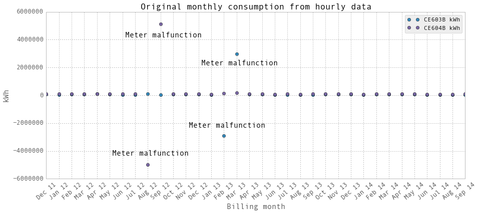
上面是使用我们的数据处理方法的每月用电量图。显然,这两个电表故障了好几个月。有两组圆点“CE603B”和“CE604B”,它们来自两个电表。有两个电表。它们的总和就是该建筑物的总耗电量。
monthlyElectricity.loc['Aug 12','CE604B kWh'] = np.nan
monthlyElectricity.loc['Sep 12','CE604B kWh'] = np.nan
monthlyElectricity.loc['Feb 13','CE603B kWh'] = np.nan
monthlyElectricity.loc['Mar 13','CE603B kWh'] = np.nan


fig,ax = plt.subplots(1, 1,figsize=(15,8))
#ax.set_axis_bgcolor('w')
plt.bar(np.arange(0, len(monthlyElectricity))-0.5,monthlyElectricity['CE603B kWh'], label='Our data processing from hourly data')
plt.plot(monthlyElectricityFromFacility.loc[months,'CE603B kWh'],'or', label='Facility data')
plt.xticks(np.arange(0,len(months)),months)
plt.xlabel('Month',fontsize=15)
plt.ylabel('kWh',fontsize=15)
plt.xlim([0, len(monthlyElectricity)])
plt.legend()
ax.set_xticklabels(months, rotation=40, fontsize=13)
plt.tick_params(which=u'major', reset=False, axis = 'y', labelsize = 15)
plt.title('Comparison between our data processing and facilities, Meter CE603B',fontsize=20)

text = 'Meter malfunction \n estimated by facility'
ax.annotate(text, xy = (14, monthlyElectricityFromFacility.loc['Feb 13','CE603B kWh']),
            xytext = (5, 50), fontsize = 15,
            arrowprops=dict(facecolor='black', shrink=0.15),
            textcoords = 'offset points', ha = 'center', va = 'bottom')

ax.annotate(text, xy = (15, monthlyElectricityFromFacility.loc['Mar 13','CE603B kWh']),
            xytext = (5, 50), fontsize = 15,
            arrowprops=dict(facecolor='black', shrink=0.15),
            textcoords = 'offset points', ha = 'center', va = 'bottom')
plt.show()

fig,ax = plt.subplots(1, 1,figsize=(15,8))
#ax.set_axis_bgcolor('w')
plt.bar(np.arange(0, len(monthlyElectricity))-0.5, monthlyElectricity['CE604B kWh'], label='Our data processing from hourly data')
plt.plot(monthlyElectricityFromFacility.loc[months,'CE604B kWh'],'or', label='Facility data')
plt.xticks(np.arange(0,len(months)),months)
plt.xlabel('Month',fontsize=15)
plt.ylabel('kWh',fontsize=15)
plt.xlim([0, len(monthlyElectricity)])
plt.legend()
ax.set_xticklabels(months, rotation=40, fontsize=13)
plt.tick_params(which=u'major', reset=False, axis = 'y', labelsize = 15)
plt.title('Comparison between our data processing and facilities, Meter CE604B',fontsize=20)


ax.annotate(text, xy = (9, monthlyElectricityFromFacility.loc['Sep 12','CE604B kWh']),
            xytext = (5, 50), fontsize = 15,
            arrowprops=dict(facecolor='black', shrink=0.15),
            textcoords = 'offset points', ha = 'center', va = 'bottom')

ax.annotate(text, xy = (8, monthlyElectricityFromFacility.loc['Aug 12','CE604B kWh']),
            xytext = (5, 50), fontsize = 15,
            arrowprops=dict(facecolor='black', shrink=0.15),
            textcoords = 'offset points', ha = 'center', va = 'bottom')
plt.show()


图中的点是设施每月提供的数据。它们是钞票上的账单。当电表发生故障时,该设施只是对表的能量消耗进行估算。我们排除的数据点不在图中。它们只是比正常水平高得多(是其他正常消费水平的30倍)。“仪表故障,设施预估”是指本月仪表出现故障,这个点是设施预估的。
2013年2月和3月,电表“CE603B”出现故障。2012年8月和9月,电表“CE604B”出现故障。我们把这几个月的关键字设为np.nan。简单地把他们排除在回归之外。再次绘制它们,并与设施月度数据进行比较。 当然,当仪表出故障时除外。在这几个月里,这些设施为了记账而估算能源消耗。对于我们来说,我们只是在回归中剔除了这些月份的每小时和每天的数据点。
建筑总用电量是这电表的总和。为了以防万一,我们把“power”和“energy”放在一起比较
electricity['energy'] = electricity['Gund Bus-A EnergyReal - kWhr'] + electricity['Gund Bus-B EnergyReal - kWhr']
electricity['power'] = electricity['Gund Bus-A PowerReal - kW'] + electricity['Gund Bus-B PowerReal - kW']
electricity.head()
| Gund Bus-A EnergyReal - kWhr | Gund Bus-B EnergyReal - kWhr | Gund Bus-A PowerReal - kW | Gund Bus-B PowerReal - kW | energy | power | startTime | endTime | |
|---|---|---|---|---|---|---|---|---|
| 2011-07-01 00:00:00 | NaN | NaN | NaN | NaN | NaN | NaN | 2011-07-01 00:00:00 | 2011-07-01 01:00:00 |
| 2011-07-01 01:00:00 | 1796757.502803 | 3657811.582122 | 47.184015 | 63.486186 | 5454569.084925 | 110.670201 | 2011-07-01 01:00:00 | 2011-07-01 02:00:00 |
| 2011-07-01 02:00:00 | 1796800.145991 | 3657873.464938 | 40.208796 | 61.270542 | 5454673.610929 | 101.479338 | 2011-07-01 02:00:00 | 2011-07-01 03:00:00 |
| 2011-07-01 03:00:00 | 1796840.146023 | 3657934.837505 | 39.209866 | 61.464394 | 5454774.983528 | 100.674260 | 2011-07-01 03:00:00 | 2011-07-01 04:00:00 |
| 2011-07-01 04:00:00 | 1796879.023607 | 3657995.470348 | 39.378507 | 59.396581 | 5454874.493955 | 98.775088 | 2011-07-01 04:00:00 | 2011-07-01 05:00:00 |
获得每小时消耗
这个小时和下一个小时之间的每小时能耗是下一个小时减去这个小时的电表kWh读数(dataframe中的“energy”)。我们假设电表读数是在一小时结束时记录的。为了避免混淆,我们还在dataframe中标记了抄表的开始时间和结束时间。我们将下一小时的每小时电量与推导出的每小时电量进行了比较,大多数时候,电量接近每小时电量。有时,会有很大的不同。
电表记录了累计能耗。假设今天一开始,数字是10。一小时后,用电量为1,然后电表号加1变成11,等等。所以仪表的数量应该不断增加。然而,我们发现,有时,水表读数突然下降到0,过了一段时间,又得到一个很高的正数。这将产生负的每小时消费,然后是一个荒谬的高正电荷数。我们用“t + 1时刻的电表读数- t时刻的电表读数”来计算每小时/每天的能源消耗。如果结果是负数,或者高得离谱,我们就认为仪表出了故障。我们把这些数据点设为np.nan。通过查看excel文件中的原始数据和每月的图表,我们计算出了仪表发生故障的确切日期。
除此之外,偶尔还会有更多的无意义数据点,它们比正常值高出一千倍。正常的小时消耗量范围在100到400之间。我们创建了一个过滤器:“index = abs(hourlyEnergy) < 200000”,这意味着只保留低于200000的值。
# 如果有任何遗漏的小时,重新索引,以获得整个时间跨度。填写nan数据。
hourlyTimestamp = pd.date_range(start = '2011/7/1', end = '2014/10/31', freq = 'H')

# 不知何故,重索引并不能很好地工作。2011年10月和其他几个小时的失踪。
# 基本上就是原始长度的长度。
# electricity.reindex(hourlyTimestamp, inplace = True, fill_value = np.nan)

startTime = hourlyTimestamp
endTime = hourlyTimestamp + np.timedelta64(1,'h')
hourlyTime = pd.DataFrame(data = np.transpose([startTime, endTime]), index = hourlyTimestamp, columns = ['startTime', 'endTime'])

electricity = electricity.join(hourlyTime, how = 'outer')

# 以防万一,为了使用diff方法,时间戳必须是按升序排列的。
electricity.sort_index(inplace = True)
hourlyEnergy = electricity.diff(periods=1)['energy']

hourlyElectricity = pd.DataFrame(data = hourlyEnergy.values, index = hourlyEnergy.index, columns = ['electricity-kWh'])
hourlyElectricity = hourlyElectricity.join(hourlyTime, how = 'inner')

print "Data length: ", len(hourlyElectricity)/24, " days"
hourlyElectricity.head()
Data length: 1218.04166667 days
| electricity-kWh | startTime | endTime | |
|---|---|---|---|
| 2011-07-01 00:00:00 | NaN | 2011-07-01 00:00:00 | 2011-07-01 01:00:00 |
| 2011-07-01 01:00:00 | NaN | 2011-07-01 01:00:00 | 2011-07-01 02:00:00 |
| 2011-07-01 02:00:00 | 104.526004 | 2011-07-01 02:00:00 | 2011-07-01 03:00:00 |
| 2011-07-01 03:00:00 | 101.372599 | 2011-07-01 03:00:00 | 2011-07-01 04:00:00 |
| 2011-07-01 04:00:00 | 99.510428 | 2011-07-01 04:00:00 | 2011-07-01 05:00:00 |
以上是小时耗电量。数据被导出到excel文件中。我们假设电表读数是在一小时结束时记录的。
# 过滤数据,保留NaN并生成两个excels,有NaN和没有NaN

hourlyElectricity.loc[abs(hourlyElectricity['electricity-kWh']) > 100000,'electricity-kWh'] = np.nan

time = hourlyElectricity.index
index = ((time > np.datetime64('2012-07-26')) & (time < np.datetime64('2012-08-18'))) \
        | ((time > np.datetime64('2013-01-21')) & (time < np.datetime64('2013-03-08')))

hourlyElectricity.loc[index,'electricity-kWh'] = np.nan
hourlyElectricityWithoutNaN = hourlyElectricity.dropna(axis=0, how='any')

hourlyElectricity.to_excel('Data/hourlyElectricity.xlsx')
hourlyElectricityWithoutNaN.to_excel('Data/hourlyElectricityWithoutNaN.xlsx')
plt.figure()
fig = hourlyElectricity.plot(fontsize = 15, figsize = (15, 6))
plt.tick_params(which=u'major', reset=False, axis = 'y', labelsize = 15)
fig.set_axis_bgcolor('w')
plt.title('All the hourly electricity data', fontsize = 16)
plt.ylabel('kWh')
plt.show()

plt.figure()
fig = hourlyElectricity.iloc[26200:27400,:].plot(marker = 'o',label='hourly electricity', fontsize = 15, figsize = (15, 6))
plt.tick_params(which=u'major', reset=False, axis = 'y', labelsize = 15)
fig.set_axis_bgcolor('w')
plt.title('Hourly electricity data of selected days', fontsize = 16)
plt.ylabel('kWh')
plt.legend()
plt.show()
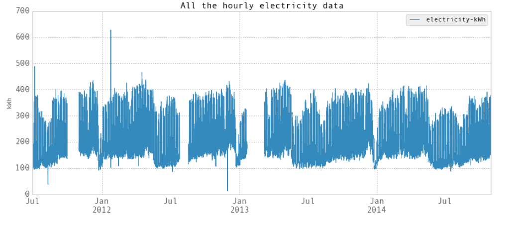
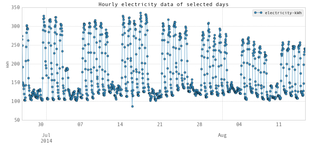
上面是每小时的数据图。在第一个图中,空白部分是由于仪表故障时数据丢失造成的。在第二张图中,你可以看到白天和晚上,工作日和周末的区别。
获得日常消耗
我们通过“reindex”来获得每天的用电量。
dailyTimestamp = pd.date_range(start = '2011/7/1', end = '2014/10/31', freq = 'D')
electricityReindexed = electricity.reindex(dailyTimestamp, inplace = False)

# 以防万一,为了使用diff方法,时间戳必须是按升序排列的。
electricityReindexed.sort_index(inplace = True)
dailyEnergy = electricityReindexed.diff(periods=1)['energy']

dailyElectricity = pd.DataFrame(data = dailyEnergy.values, index = electricityReindexed.index - np.timedelta64(1,'D'), columns = ['electricity-kWh'])
dailyElectricity['startDay'] = dailyElectricity.index
dailyElectricity['endDay'] = dailyElectricity.index + np.timedelta64(1,'D')

# 过滤数据,保留NaN并生成两个excels,有NaN和没有NaN
dailyElectricity.loc[abs(dailyElectricity['electricity-kWh']) > 2000000,'electricity-kWh'] = np.nan

time = dailyElectricity.index
index = ((time > np.datetime64('2012-07-26')) & (time < np.datetime64('2012-08-18'))) | ((time > np.datetime64('2013-01-21')) & (time < np.datetime64('2013-03-08')))

dailyElectricity.loc[index,'electricity-kWh'] = np.nan
dailyElectricityWithoutNaN = dailyElectricity.dropna(axis=0, how='any')

dailyElectricity.to_excel('Data/dailyElectricity.xlsx')
dailyElectricityWithoutNaN.to_excel('Data/dailyElectricityWithoutNaN.xlsx')

dailyElectricity.head()
| electricity-kWh | startDay | endDay | |
|---|---|---|---|
| 2011-06-30 | NaN | 2011-06-30 | 2011-07-01 |
| 2011-07-01 | NaN | 2011-07-01 | 2011-07-02 |
| 2011-07-02 | 3630.398480 | 2011-07-02 | 2011-07-03 |
| 2011-07-03 | 3750.648885 | 2011-07-03 | 2011-07-04 |
| 2011-07-04 | 4568.724044 | 2011-07-04 | 2011-07-05 |
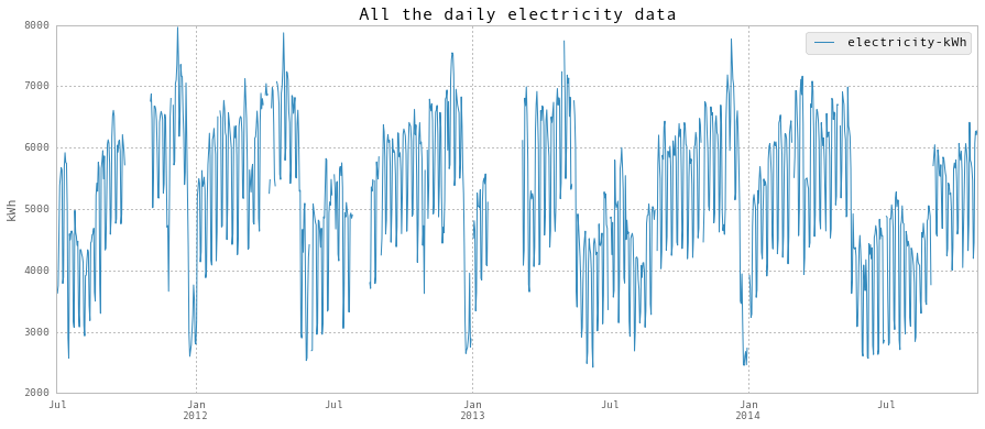
以上是日用电量。
plt.figure()
fig = dailyElectricity.plot(figsize = (15, 6))
fig.set_axis_bgcolor('w')
plt.title('All the daily electricity data', fontsize = 16)
plt.ylabel('kWh')
plt.show()

plt.figure()
fig = dailyElectricity.iloc[1000:1130,:].plot(marker = 'o', figsize = (15, 6))
fig.set_axis_bgcolor('w')
plt.title('Daily electricity data of selected days', fontsize = 16)
plt.ylabel('kWh')
plt.show()

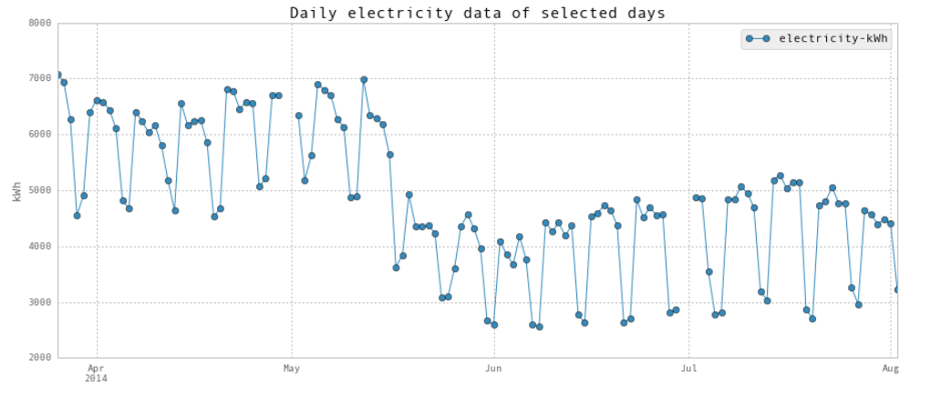
上面是每日电量图。
超低耗电量发生在学期结束后,包括圣诞节假期。另外,如图2所示,开学时夏季的能耗较低。
冷水
我们处理冷水数据的方式与电力相同。
chilledWater = df[['Gund Main Energy - Ton-Days']]
chilledWater.head()
| Gund Main Energy - Ton-Days | |
|---|---|
| 2011-07-01 01:00:00 | 17912.537804 |
| 2011-07-01 02:00:00 | 17912.853518 |
| 2011-07-01 03:00:00 | 17913.169232 |
| 2011-07-01 04:00:00 | 17913.484946 |
| 2011-07-01 05:00:00 | 17913.800660 |
file = 'Data/monthly chilled water.csv'
monthlyChilledWaterFromFacility = pd.read_csv(file, header=0)
monthlyChilledWaterFromFacility.set_index(['month'], inplace = True)
monthlyChilledWaterFromFacility.head()
| startDate | endDate | chilledWater | |
|---|---|---|---|
| month | |||
| 11-Jul | 6/12/11 | 7/12/11 | 2258 |
| 11-Aug | 7/12/11 | 8/12/11 | 2095 |
| 11-Sep | 8/12/11 | 9/12/11 | 2200 |
| 11-Oct | 9/12/11 | 10/12/11 | 1664 |
| 11-Nov | 10/12/11 | 11/12/11 | 447 |
monthlyChilledWaterFromFacility['startDate'] = pd.to_datetime(monthlyChilledWaterFromFacility['startDate'], format="%m/%d/%y")
values = monthlyChilledWaterFromFacility.index.values
keys = np.array(monthlyChilledWaterFromFacility['startDate'])
dates = {}
for key, value in zip(keys, values):
dates[key] = value
sortedDates = np.sort(dates.keys())
sortedDates = sortedDates[sortedDates > np.datetime64('2011-11-01')]
months = []
monthlyChilledWaterOrg = np.zeros((len(sortedDates) - 1))
for i in range(len(sortedDates) - 1):
begin = sortedDates[i]
end = sortedDates[i+1]
months.append(dates[sortedDates[i]])
monthlyChilledWaterOrg[i] = (np.round(chilledWater.loc[end,:] - chilledWater.loc[begin,:], 1))
monthlyChilledWater = pd.DataFrame(data = monthlyChilledWaterOrg, index = months, columns = ['chilledWater-TonDays'])
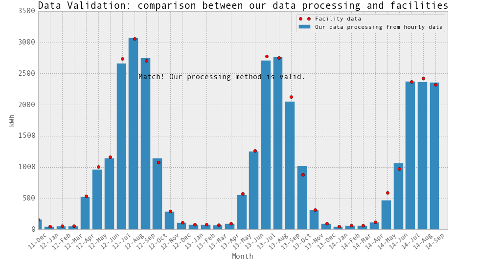
fig,ax = plt.subplots(1, 1,figsize=(15,8))
#ax.set_axis_bgcolor('w')
#plt.plot(monthlyChilledWater, label='Our data processing from hourly data', marker = 'x', markersize = 15, linestyle = '')
plt.bar(np.arange(len(monthlyChilledWater))-0.5, monthlyChilledWater.values, label='Our data processing from hourly data')
plt.plot(monthlyChilledWaterFromFacility[5:-1]['chilledWater'],'or', label='Facility data')
plt.xticks(np.arange(0,len(months)),months)
plt.xlabel('Month',fontsize=15)
plt.ylabel('kWh',fontsize=15)
plt.xlim([0,len(months)])
plt.legend()
ax.set_xticklabels(months, rotation=40, fontsize=13)
plt.tick_params(which=u'major', reset=False, axis = 'y', labelsize = 15)
plt.title('Data Validation: comparison between our data processing and facilities',fontsize=20)
text = 'Match! Our processing method is valid.'
ax.annotate(text, xy = (15, 2000),
xytext = (5, 50), fontsize = 15,
textcoords = 'offset points', ha = 'center', va = 'bottom')
plt.show()
。
hourlyTimestamp = pd.date_range(start = '2011/7/1', end = '2014/10/31', freq = 'H')
chilledWater.reindex(hourlyTimestamp, inplace = True)

# 以防万一,为了使用diff方法,时间戳必须是按升序排列的。
chilledWater.sort_index(inplace = True)
hourlyEnergy = chilledWater.diff(periods=1)

hourlyChilledWater = pd.DataFrame(data = hourlyEnergy.values, index = hourlyEnergy.index, columns = ['chilledWater-TonDays'])
hourlyChilledWater['startTime'] = hourlyChilledWater.index
hourlyChilledWater['endTime'] = hourlyChilledWater.index + np.timedelta64(1,'h')

hourlyChilledWater.loc[abs(hourlyChilledWater['chilledWater-TonDays']) > 50,'chilledWater-TonDays'] = np.nan

hourlyChilledWaterWithoutNaN = hourlyChilledWater.dropna(axis=0, how='any')

hourlyChilledWater.to_excel('Data/hourlyChilledWater.xlsx')
hourlyChilledWaterWithoutNaN.to_excel('Data/hourlyChilledWaterWithoutNaN.xlsx')

plt.figure()
fig = hourlyChilledWater.plot(fontsize = 15, figsize = (15, 6))
plt.tick_params(which=u'major', reset=False, axis = 'y', labelsize = 15)
fig.set_axis_bgcolor('w')
plt.title('All the hourly chilled water data', fontsize = 16)
plt.ylabel('Ton-Days')
plt.show()

hourlyChilledWater.head()

| chilledWater-TonDays | startTime | endTime | |
|---|---|---|---|
| 2011-07-01 01:00:00 | NaN | 2011-07-01 01:00:00 | 2011-07-01 02:00:00 |
| 2011-07-01 02:00:00 | 0.315714 | 2011-07-01 02:00:00 | 2011-07-01 03:00:00 |
| 2011-07-01 03:00:00 | 0.315714 | 2011-07-01 03:00:00 | 2011-07-01 04:00:00 |
| 2011-07-01 04:00:00 | 0.315714 | 2011-07-01 04:00:00 | 2011-07-01 05:00:00 |
| 2011-07-01 05:00:00 | 0.315714 | 2011-07-01 05:00:00 | 2011-07-01 06:00:00 |
dailyTimestamp = pd.date_range(start = '2011/7/1', end = '2014/10/31', freq = 'D')
chilledWaterReindexed = chilledWater.reindex(dailyTimestamp, inplace = False)
chilledWaterReindexed.sort_index(inplace = True)
dailyEnergy = chilledWaterReindexed.diff(periods=1)['Gund Main Energy - Ton-Days']
dailyChilledWater = pd.DataFrame(data = dailyEnergy.values, index = chilledWaterReindexed.index - np.timedelta64(1,'D'), columns = ['chilledWater-TonDays'])
dailyChilledWater['startDay'] = dailyChilledWater.index
dailyChilledWater['endDay'] = dailyChilledWater.index + np.timedelta64(1,'D')
dailyChilledWaterWithoutNaN = dailyChilledWater.dropna(axis=0, how='any')
dailyChilledWater.to_excel('Data/dailyChilledWater.xlsx')
dailyChilledWaterWithoutNaN.to_excel('Data/dailyChilledWaterWithoutNaN.xlsx')
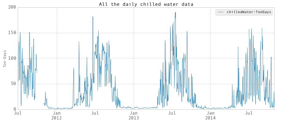
plt.figure()
fig = dailyChilledWater.plot(fontsize = 15, figsize = (15, 6))
plt.tick_params(which=u'major', reset=False, axis = 'y', labelsize = 15)
fig.set_axis_bgcolor('w')
plt.title('All the daily chilled water data', fontsize = 16)
plt.ylabel('Ton-Days')
plt.show()
dailyChilledWater.head()
| chilledWater-TonDays | startDay | endDay | |
|---|---|---|---|
| 2011-06-30 | NaN | 2011-06-30 | 2011-07-01 |
| 2011-07-01 | NaN | 2011-07-01 | 2011-07-02 |
| 2011-07-02 | 54.741028 | 2011-07-02 | 2011-07-03 |
| 2011-07-03 | 55.649728 | 2011-07-03 | 2011-07-04 |
| 2011-07-04 | 109.049077 | 2011-07-04 | 2011-07-05 |
热水
steam = df[['Gund Condensate FlowTotal - LBS']]
steam.head()
| Gund Condensate FlowTotal - LBS | |
|---|---|
| 2011-07-01 01:00:00 | 15443350.388455 |
| 2011-07-01 02:00:00 | 15443459.322917 |
| 2011-07-01 03:00:00 | 15443574.687500 |
| 2011-07-01 04:00:00 | 15443701.953125 |
| 2011-07-01 05:00:00 | 15443818.359375 |
file = 'Data/monthly steam.csv'
monthlySteamFromFacility = pd.read_csv(file, header=0)
monthlySteamFromFacility.set_index(['month'], inplace = True)
monthlySteamFromFacility.head()
| startDate | endDate | steam | |
|---|---|---|---|
| month | |||
| Jul 11 | 6/17/2011 | 7/21/2011 | 0.0 |
| Aug 11 | 7/21/2011 | 8/20/2011 | 0.0 |
| Sep 11 | 8/20/2011 | 9/17/2011 | 0.0 |
| Oct 11 | 9/17/2011 | 10/20/2011 | 246.5 |
| Nov 11 | 10/20/2011 | 11/20/2011 | 786.1 |
monthlySteamFromFacility['startDate'] = pd.to_datetime(monthlySteamFromFacility['startDate'], format="%m/%d/%Y")
values = monthlySteamFromFacility.index.values

keys = np.array(monthlySteamFromFacility['startDate'])

dates = {}
for key, value in zip(keys, values):
    dates[key] = value

sortedDates =  np.sort(dates.keys())
sortedDates = sortedDates[sortedDates > np.datetime64('2011-11-01')]

months = []
monthlySteamOrg = np.zeros((len(sortedDates) - 1))
for i in range(len(sortedDates) - 1):
    begin = sortedDates[i]
    end = sortedDates[i+1]
    months.append(dates[sortedDates[i]])
    monthlySteamOrg[i] = (np.round(steam.loc[end,:] -  steam.loc[begin,:], 1))


monthlySteam = pd.DataFrame(data = monthlySteamOrg, index = months, columns = ['steam-LBS'])

# 867 LBS ~= 1MMBTU steam

fig,ax = plt.subplots(1, 1,figsize=(15,8))
#ax.set_axis_bgcolor('w')
#plt.plot(monthlySteam/867, label='Our data processing from hourly data')
plt.bar(np.arange(len(monthlySteam))-0.5, monthlySteam.values/867, label='Our data processing from hourly data')
plt.plot(monthlySteamFromFacility.loc[months,'steam'],'or', label='Facility data')
plt.xticks(np.arange(0,len(months)),months)
plt.xlabel('Month',fontsize=15)
plt.ylabel('Steam (MMBTU)',fontsize=15)
plt.xlim([0,len(months)])
plt.legend()
ax.set_xticklabels(months, rotation=40, fontsize=13)
plt.tick_params(which=u'major', reset=False, axis = 'y', labelsize = 15)
plt.title('Comparison between our data processing and facilities - Steam',fontsize=20)

text = 'Match! Our processing method is valid.'
ax.annotate(text, xy = (9, 1500),
            xytext = (5, 50), fontsize = 15,
            textcoords = 'offset points', ha = 'center', va = 'bottom')

plt.show()
hourlyTimestamp = pd.date_range(start = '2011/7/1', end = '2014/10/31', freq = 'H')
steam.reindex(hourlyTimestamp, inplace = True)

# Just in case, in order to use diff method, timestamp has to be in asending order.
steam.sort_index(inplace = True)
hourlyEnergy = steam.diff(periods=1)

hourlySteam = pd.DataFrame(data = hourlyEnergy.values, index = hourlyEnergy.index, columns = ['steam-LBS'])
hourlySteam['startTime'] = hourlySteam.index
hourlySteam['endTime'] = hourlySteam.index + np.timedelta64(1,'h')

hourlySteam.loc[abs(hourlySteam['steam-LBS']) > 100000,'steam-LBS'] = np.nan

plt.figure()
fig = hourlySteam.plot(fontsize = 15, figsize = (15, 6))
plt.tick_params(which=u'major', reset=False, axis = 'y', labelsize = 17)
fig.set_axis_bgcolor('w')
plt.title('All the hourly steam data', fontsize = 16)
plt.ylabel('LBS')
plt.show()

hourlySteamWithoutNaN = hourlySteam.dropna(axis=0, how='any')

hourlySteam.to_excel('Data/hourlySteam.xlsx')
hourlySteamWithoutNaN.to_excel('Data/hourlySteamWithoutNaN.xlsx')

hourlySteam.head()

| steam-LBS | startTime | endTime | |
|---|---|---|---|
| 2011-07-01 01:00:00 | NaN | 2011-07-01 01:00:00 | 2011-07-01 02:00:00 |
| 2011-07-01 02:00:00 | 108.934462 | 2011-07-01 02:00:00 | 2011-07-01 03:00:00 |
| 2011-07-01 03:00:00 | 115.364583 | 2011-07-01 03:00:00 | 2011-07-01 04:00:00 |
| 2011-07-01 04:00:00 | 127.265625 | 2011-07-01 04:00:00 | 2011-07-01 05:00:00 |
| 2011-07-01 05:00:00 | 116.406250 | 2011-07-01 05:00:00 | 2011-07-01 06:00:00 |
dailyTimestamp = pd.date_range(start = '2011/7/1', end = '2014/10/31', freq = 'D')
steamReindexed = steam.reindex(dailyTimestamp, inplace = False)

steamReindexed.sort_index(inplace = True)
dailyEnergy = steamReindexed.diff(periods=1)['Gund Condensate FlowTotal - LBS']

dailySteam = pd.DataFrame(data = dailyEnergy.values, index = steamReindexed.index - np.timedelta64(1,'D'), columns = ['steam-LBS'])
dailySteam['startDay'] = dailySteam.index
dailySteam['endDay'] = dailySteam.index + np.timedelta64(1,'D')

plt.figure()
fig = dailySteam.plot(fontsize = 15, figsize = (15, 6))
plt.tick_params(which=u'major', reset=False, axis = 'y', labelsize = 15)
fig.set_axis_bgcolor('w')
plt.title('All the daily steam data', fontsize = 16)
plt.ylabel('LBS')
plt.show()

dailySteamWithoutNaN = dailyChilledWater.dropna(axis=0, how='any')

dailySteam.to_excel('Data/dailySteam.xlsx')
dailySteamWithoutNaN.to_excel('Data/dailySteamWithoutNaN.xlsx')

dailySteam.head()
| steam-LBS | startDay | endDay | |
|---|---|---|---|
| 2011-06-30 | NaN | 2011-06-30 | 2011-07-01 |
| 2011-07-01 | NaN | 2011-07-01 | 2011-07-02 |
| 2011-07-02 | 3250.651042 | 2011-07-02 | 2011-07-03 |
| 2011-07-03 | 3271.276042 | 2011-07-03 | 2011-07-04 |
| 2011-07-04 | 3236.718750 | 2011-07-04 | 2011-07-05 |
天气数据
原始数据
天气有两个数据源。
- 2014年: GSD(设计研究生院)楼顶上的天气。
- 2012 & 2013年: 从位于Cambridge, MA的气象站购买天气数据。请注意,2012年和2013年的数据来自不同的气象站。
这是经过一些清洗后的原始天气数据,包括单位转换。间隔是5分钟。
weather2014 = pd.read_excel('Data/weather-2014.xlsx')
weather2014.head()
| Datetime | T-C | RH-% | Tdew-C | windDirection | windSpeed-m/s | pressure-mbar | solarRadiation-W/m2 | |
|---|---|---|---|---|---|---|---|---|
| 0 | 2014-01-01 00:00:00 | -5.02 | 53.2 | -13.07 | 256 | 4.5 | 1020.8 | 1 |
| 1 | 2014-01-01 00:05:00 | -5.14 | 54.3 | -12.93 | 257 | 4.0 | 1020.7 | 1 |
| 2 | 2014-01-01 00:10:00 | -5.08 | 53.4 | -13.08 | 258 | 3.5 | 1021.1 | 1 |
| 3 | 2014-01-01 00:15:00 | -5.17 | 52.6 | -13.35 | 257 | 2.8 | 1021.0 | 1 |
| 4 | 2014-01-01 00:20:00 | -5.23 | 52.9 | -13.33 | 248 | 2.5 | 1021.2 | 1 |
通过重采样方法转换为每小时一次。
这是2014年每小时的天气数据。
weather2014 = weather2014.set_index('Datetime')
weather2014 = weather2014.resample('H')
weather2014.head()
| T-C | RH-% | Tdew-C | windDirection | windSpeed-m/s | pressure-mbar | solarRadiation-W/m2 | |
|---|---|---|---|---|---|---|---|
| Datetime | |||||||
| 2014-01-01 00:00:00 | -5.281667 | 52.858333 | -13.393333 | 253.500000 | 2.775000 | 1021.158333 | 1 |
| 2014-01-01 01:00:00 | -5.725000 | 51.650000 | -14.090833 | 253.000000 | 2.350000 | 1021.700000 | 1 |
| 2014-01-01 02:00:00 | -6.002500 | 50.766667 | -14.555833 | 239.250000 | 1.133333 | 1022.708333 | 1 |
| 2014-01-01 03:00:00 | -6.320833 | 49.675000 | -15.114167 | 234.333333 | 1.191667 | 1023.233333 | 1 |
| 2014-01-01 04:00:00 | -6.535833 | 49.708333 | -15.305833 | 227.333333 | 1.633333 | 1023.925000 | 1 |
这里是2013年和2014年的原始天气数据,经过一些清洗,包括单位转换。可以看出,Datetime格式不正确。
weather2012and2013 = pd.read_excel('Data/weather-2012-2013.xlsx')
weather2012and2013.head()
| Datetime | RH-% | windDirection | solarRadiation-W/m2 | T-C | Tdew-C | pressure-mbar | windSpeed-m/s | |
|---|---|---|---|---|---|---|---|---|
| 0 | 2012-01-01-01 | 87 | 310 | 0 | 4 | 1.9 | 1004 | 4.166670 |
| 1 | 2012-01-01-02 | 87 | 280 | 0 | 4 | 1.9 | 1005 | 4.166670 |
| 2 | 2012-01-01-03 | 81 | 270 | 0 | 5 | 1.9 | 1006 | 4.166670 |
| 3 | 2012-01-01-04 | 76 | 290 | 0 | 6 | 1.9 | 1007 | 4.722226 |
| 4 | 2012-01-01-05 | 87 | 280 | 0 | 4 | 1.9 | 1007 | 3.055558 |
这是清洗后每小时的数据。
weather2012and2013['Datetime'] = pd.to_datetime(weather2012and2013['Datetime'], format='%Y-%m-%d-%H')
weather2012and2013 = weather2012and2013.set_index('Datetime')
weather2012and2013.head()
| RH-% | windDirection | solarRadiation-W/m2 | T-C | Tdew-C | pressure-mbar | windSpeed-m/s | |
|---|---|---|---|---|---|---|---|
| Datetime | |||||||
| 2012-01-01 01:00:00 | 87 | 310 | 0 | 4 | 1.9 | 1004 | 4.166670 |
| 2012-01-01 02:00:00 | 87 | 280 | 0 | 4 | 1.9 | 1005 | 4.166670 |
| 2012-01-01 03:00:00 | 81 | 270 | 0 | 5 | 1.9 | 1006 | 4.166670 |
| 2012-01-01 04:00:00 | 76 | 290 | 0 | 6 | 1.9 | 1007 | 4.722226 |
| 2012-01-01 05:00:00 | 87 | 280 | 0 | 4 | 1.9 | 1007 | 3.055558 |
每小时天气数据
合并两个文件,增加更多的功能,包括冷度,热度,湿度比和除湿。
这是每小时的天气数据。
# 合并两个天气文件
hourlyWeather = weather2014.append(weather2012and2013)
hourlyWeather.index.name = None
hourlyWeather.sort_index(inplace = True)

# 增加更多的特征
# 将相对湿度转换为相对湿度

Mw=18.0160 # 水的分子量
Md=28.9660 # 干燥空气的分子量
R =  8.31432E3 # 气体常数
Rd = R/Md # 干燥空气的比气体常数
Rv = R/Mw # 蒸汽的比气体常数
Lv = 2.5e6 # 水蒸气凝结放热[J kg-1]
eps = Mw/Md

# 饱和压力
def esat(T):
    ''' 给定空气温度(单位[K]),得到给定压力(单位[Pa]) '''
    from numpy import log10
    TK = 273.15
    e1 = 101325.0
    logTTK = log10(T/TK)
    esat =  e1*10**(10.79586*(1-TK/T)-5.02808*logTTK+ 1.50474*1e-4*(1.-10**(-8.29692*(T/TK-1)))+ 0.42873*1e-3*(10**(4.76955*(1-TK/T))-1)-2.2195983)
    return esat

def rh2sh(RH,p,T):
    '''用途:将相对湿度(无单位)换算成比湿度(湿度比)[kg/kg]'''
    es = esat(T)
    W = Mw/Md*RH*es/(p-RH*es)

    return W/(1.+W)


p = hourlyWeather['pressure-mbar'] * 100
RH = hourlyWeather['RH-%'] / 100
T = hourlyWeather['T-C'] + 273.15
w = rh2sh(RH,p,T)

hourlyWeather['humidityRatio-kg/kg'] = w
hourlyWeather['coolingDegrees'] = hourlyWeather['T-C'] - 12
hourlyWeather.loc[hourlyWeather['coolingDegrees'] < 0, 'coolingDegrees'] = 0

hourlyWeather['heatingDegrees'] = 15 - hourlyWeather['T-C']
hourlyWeather.loc[hourlyWeather['heatingDegrees'] < 0, 'heatingDegrees'] = 0

hourlyWeather['dehumidification'] = hourlyWeather['humidityRatio-kg/kg'] - 0.00886
hourlyWeather.loc[hourlyWeather['dehumidification'] < 0, 'dehumidification'] = 0

#hourlyWeather.to_excel('Data/hourlyWeather.xlsx')
hourlyWeather.head()
| RH-% | T-C | Tdew-C | pressure-mbar | solarRadiation-W/m2 | windDirection | windSpeed-m/s | humidityRatio-kg/kg | coolingDegrees | heatingDegrees | dehumidification | |
|---|---|---|---|---|---|---|---|---|---|---|---|
| 2012-01-01 01:00:00 | 87 | 4 | 1.9 | 1004 | 0 | 310 | 4.166670 | 0.004396 | 0 | 11 | 0 |
| 2012-01-01 02:00:00 | 87 | 4 | 1.9 | 1005 | 0 | 280 | 4.166670 | 0.004391 | 0 | 11 | 0 |
| 2012-01-01 03:00:00 | 81 | 5 | 1.9 | 1006 | 0 | 270 | 4.166670 | 0.004380 | 0 | 10 | 0 |
| 2012-01-01 04:00:00 | 76 | 6 | 1.9 | 1007 | 0 | 290 | 4.722226 | 0.004401 | 0 | 9 | 0 |
| 2012-01-01 05:00:00 | 87 | 4 | 1.9 | 1007 | 0 | 280 | 3.055558 | 0.004382 | 0 | 11 | 0 |
plt.figure()
fig = hourlyWeather.plot(y = 'T-C', figsize = (15, 6))
fig.set_axis_bgcolor('w')
plt.title('All hourly temperture', fontsize = 16)
plt.ylabel(r'Temperature ($\circ$C)')
plt.show()
plt.figure()
fig = hourlyWeather.plot(y = 'solarRadiation-W/m2', figsize = (15, 6))
fig.set_axis_bgcolor('w')
plt.title('All hourly solar radiation', fontsize = 16)
plt.ylabel(r'$W/m^2$', fontsize = 13)
plt.show()
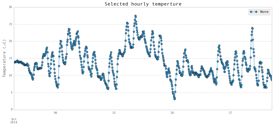
plt.figure()
fig = hourlyWeather['2014-10'].plot(y = 'T-C', figsize = (15, 6), marker = 'o')
fig.set_axis_bgcolor('w')
plt.title('Selected hourly temperture',fontsize = 16)
plt.ylabel(r'Temperature ($\circ$C)',fontsize = 13)
plt.show()
plt.figure()
fig = hourlyWeather['2014-10'].plot(y = 'solarRadiation-W/m2', figsize = (15, 6), marker ='o')
fig.set_axis_bgcolor('w')
plt.title('Selected hourly solar radiation', fontsize = 16)
plt.ylabel(r'$W/m^2$', fontsize = 13)
plt.show()


每天的天气数据
dailyWeather = hourlyWeather.resample('D')
#dailyWeather.to_excel('Data/dailyWeather.xlsx')
dailyWeather.head()
| RH-% | T-C | Tdew-C | pressure-mbar | solarRadiation-W/m2 | windDirection | windSpeed-m/s | humidityRatio-kg/kg | coolingDegrees | heatingDegrees | dehumidification | |
|---|---|---|---|---|---|---|---|---|---|---|---|
| 2012-01-01 | 76.652174 | 7.173913 | 3.073913 | 1004.956522 | 95.260870 | 236.086957 | 4.118361 | 0.004796 | 0 | 7.826087 | 0 |
| 2012-01-02 | 55.958333 | 5.833333 | -2.937500 | 994.625000 | 87.333333 | 253.750000 | 5.914357 | 0.003415 | 0 | 9.166667 | 0 |
| 2012-01-03 | 42.500000 | -3.208333 | -12.975000 | 1002.125000 | 95.708333 | 302.916667 | 6.250005 | 0.001327 | 0 | 18.208333 | 0 |
| 2012-01-04 | 41.541667 | -7.083333 | -16.958333 | 1008.250000 | 98.750000 | 286.666667 | 5.127319 | 0.000890 | 0 | 22.083333 | 0 |
| 2012-01-05 | 46.916667 | -0.583333 | -9.866667 | 1002.041667 | 90.750000 | 258.333333 | 5.162041 | 0.001746 | 0 | 15.583333 | 0 |
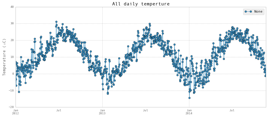
plt.figure()
fig = dailyWeather.plot(y = 'T-C', figsize = (15, 6), marker ='o')
fig.set_axis_bgcolor('w')
plt.title('All daily temperture', fontsize = 16)
plt.ylabel(r'Temperature ($\circ$C)', fontsize = 13)
plt.show()
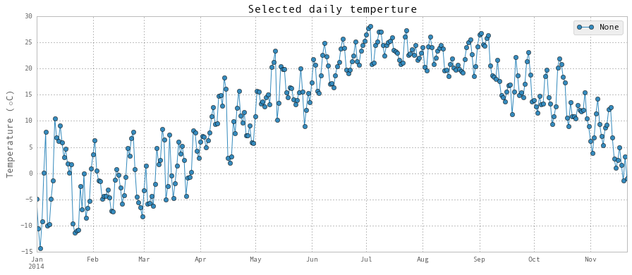
plt.figure()
fig = dailyWeather['2014'].plot(y = 'T-C', figsize = (15, 6), marker ='o')
fig.set_axis_bgcolor('w')
plt.title('Selected daily temperture', fontsize = 16)
plt.ylabel(r'Temperature ($\circ$C)', fontsize = 13)
plt.show()
plt.figure()
fig = dailyWeather['2014'].plot(y = 'solarRadiation-W/m2', figsize = (15, 6), marker ='o')
fig.set_axis_bgcolor('w')
plt.title('Selected daily solar radiation', fontsize = 16)
plt.ylabel(r'$W/m^2$', fontsize = 14)
plt.show()

与占用有关的特征
这是一个0到1之间的数。0表示无人居住,1表示正常居住。这是一个基于假期、周末和学校学术日历的估计。
holidays = pd.read_excel('Data/holidays.xlsx')
holidays.head()
| startDate | endDate | value | |
|---|---|---|---|
| 0 | 2011-07-01 | 2011-09-06 | 0.5 |
| 1 | 2011-10-10 | 2011-10-11 | 0.6 |
| 2 | 2011-11-24 | 2011-11-28 | 0.2 |
| 3 | 2011-12-22 | 2011-12-24 | 0.1 |
| 4 | 2011-12-24 | 2012-01-02 | 0.0 |
hourlyTimestamp = pd.date_range(start = '2011/7/1', end = '2014/10/31', freq = 'H')
occupancy = np.ones(len(hourlyTimestamp))

hourlyOccupancy = pd.DataFrame(data = occupancy, index = hourlyTimestamp, columns = ['occupancy'])


Saturdays = hourlyOccupancy.index.weekday == 5
Sundays = hourlyOccupancy.index.weekday == 6
hourlyOccupancy.loc[Saturdays, 'occupancy'] = 0.5
hourlyOccupancy.loc[Sundays, 'occupancy'] = 0.5


for i in range(len(holidays)):
    timestamp = pd.date_range(start = holidays.loc[i, 'startDate'], end = holidays.loc[i, 'endDate'], freq = 'H')
    hourlyOccupancy.loc[timestamp, 'occupancy'] = holidays.loc[i, 'value']

#hourlyHolidays['Datetime'] = pd.to_datetime(hourlyHolidays['Datetime'], format="%Y-%m-%d %H:%M:%S")
hourlyOccupancy['cosHour'] = np.cos((hourlyOccupancy.index.hour - 3) * 2 * np.pi / 24)

dailyOccupancy = hourlyOccupancy.resample('D')
dailyOccupancy.drop('cosHour', axis = 1, inplace = True)
合并能源消耗数据与天气和占用特征
hourlyElectricityWithFeatures = hourlyElectricity.join(hourlyWeather, how = 'inner')
hourlyElectricityWithFeatures = hourlyElectricityWithFeatures.join(hourlyOccupancy, how = 'inner')
hourlyElectricityWithFeatures.dropna(axis=0, how='any', inplace = True)
hourlyElectricityWithFeatures.to_excel('Data/hourlyElectricityWithFeatures.xlsx')
hourlyElectricityWithFeatures.head()
| electricity-kWh | startTime | endTime | RH-% | T-C | Tdew-C | pressure-mbar | solarRadiation-W/m2 | windDirection | windSpeed-m/s | humidityRatio-kg/kg | coolingDegrees | heatingDegrees | dehumidification | occupancy | cosHour | |
|---|---|---|---|---|---|---|---|---|---|---|---|---|---|---|---|---|
| 2012-01-01 01:00:00 | 111.479277 | 2012-01-01 01:00:00 | 2012-01-01 02:00:00 | 87 | 4 | 1.9 | 1004 | 0 | 310 | 4.166670 | 0.004396 | 0 | 11 | 0 | 0 | 0.866025 |
| 2012-01-01 02:00:00 | 117.989395 | 2012-01-01 02:00:00 | 2012-01-01 03:00:00 | 87 | 4 | 1.9 | 1005 | 0 | 280 | 4.166670 | 0.004391 | 0 | 11 | 0 | 0 | 0.965926 |
| 2012-01-01 03:00:00 | 119.010131 | 2012-01-01 03:00:00 | 2012-01-01 04:00:00 | 81 | 5 | 1.9 | 1006 | 0 | 270 | 4.166670 | 0.004380 | 0 | 10 | 0 | 0 | 1.000000 |
| 2012-01-01 04:00:00 | 116.005587 | 2012-01-01 04:00:00 | 2012-01-01 05:00:00 | 76 | 6 | 1.9 | 1007 | 0 | 290 | 4.722226 | 0.004401 | 0 | 9 | 0 | 0 | 0.965926 |
| 2012-01-01 05:00:00 | 111.132977 | 2012-01-01 05:00:00 | 2012-01-01 06:00:00 | 87 | 4 | 1.9 | 1007 | 0 | 280 | 3.055558 | 0.004382 | 0 | 11 | 0 | 0 | 0.866025 |
hourlyChilledWaterWithFeatures = hourlyChilledWater.join(hourlyWeather, how = 'inner')
hourlyChilledWaterWithFeatures = hourlyChilledWaterWithFeatures.join(hourlyOccupancy, how = 'inner')
hourlyChilledWaterWithFeatures.dropna(axis=0, how='any', inplace = True)
hourlyChilledWaterWithFeatures.to_excel('Data/hourlyChilledWaterWithFeatures.xlsx')

hourlySteamWithFeatures = hourlySteam.join(hourlyWeather, how = 'inner')
hourlySteamWithFeatures = hourlySteamWithFeatures.join(hourlyOccupancy, how = 'inner')
hourlySteamWithFeatures.dropna(axis=0, how='any', inplace = True)
hourlySteamWithFeatures.to_excel('Data/hourlySteamWithFeatures.xlsx')

dailyElectricityWithFeatures = dailyElectricity.join(dailyWeather, how = 'inner')
dailyElectricityWithFeatures = dailyElectricityWithFeatures.join(dailyOccupancy, how = 'inner')
dailyElectricityWithFeatures.dropna(axis=0, how='any', inplace = True)
dailyElectricityWithFeatures.to_excel('Data/dailyElectricityWithFeatures.xlsx')

dailyChilledWaterWithFeatures = dailyChilledWater.join(dailyWeather, how = 'inner')
dailyChilledWaterWithFeatures = dailyChilledWaterWithFeatures.join(dailyOccupancy, how = 'inner')
dailyChilledWaterWithFeatures.dropna(axis=0, how='any', inplace = True)
dailyChilledWaterWithFeatures.to_excel('Data/dailyChilledWaterWithFeatures.xlsx')

dailySteamWithFeatures = dailySteam.join(dailyWeather, how = 'inner')
dailySteamWithFeatures = dailySteamWithFeatures.join(dailyOccupancy, how = 'inner')
dailySteamWithFeatures.dropna(axis=0, how='any', inplace = True)
dailySteamWithFeatures.to_excel('Data/dailySteamWithFeatures.xlsx')
特性说明
命名法(按字母顺序)
coolingDegrees: 如果T-C - 12>0,则为T-C-12,否则为0。假设当室外温度低于12C时,不需要冷却,这对许多建筑来说是真实的。这对于每天的预测是有用的,因为每小时的平均冷却度比每小时的平均温度要好。
cosHour: cos(hourOfDay⋅2𝜋24)cos(hourOfDay⋅2π24)
dehumidification: 如果humidityRatio - 0.00886 > 0,则为humidityRatio - 0.00886,否则为 0。这将有助于冷水预测,特别是日常冷水预测。
heatingDegrees: 如果15 - T-C >0,则为 15 - T-C,否则为 0。假设室外温度高于15C时,不需要加热。这对于每日的预测是有用的,因为每小时的平均加热度要比每小时的平均温度好。
occupancy: 介于0和1之间的数字。0表示无人居住,1表示正常居住。这是一个基于假期、周末和学校学术日历的估计。
pressure-mbar: 大气压力
RH-% : 相对湿度
T-C : Dry-bulb 温度
Tdew-C : Dew-point 温度
湿度
湿度比是预测冷水的重要因素,因为冷水也用于干燥排到房间里的空气。使用湿度比比使用相对湿度和露点温度更有效。
%matplotlib inline

import requests
from StringIO import StringIO
import numpy as np
import pandas as pd # pandas
import matplotlib.pyplot as plt # module for plotting
import datetime as dt # module for manipulating dates and times
import numpy.linalg as lin # module for performing linear algebra operations
from __future__ import division
import matplotlib

pd.options.display.mpl_style = 'default'
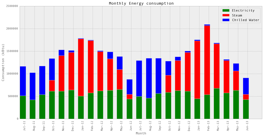
每月能源消耗
pd.options.display.mpl_style = 'default'
consumption = pd.read_csv('Data/Monthly_Energy_Gund.csv')
for i in range(len(consumption)):
    consumption['CW-kBtu'][i] = float(consumption['CW-kBtu'].values[i].replace(',', ''))
    consumption['EL-kBtu'][i] = float(consumption['EL-kBtu'].values[i].replace(',', ''))
    consumption['ST-kBtu'][i] = float(consumption['ST-kBtu'].values[i].replace(',', ''))

time_index = np.arange(len(consumption))
plt.figure(figsize=(15,7))
b1 = plt.bar(time_index, consumption['EL-kBtu'], width = 0.6, color='g')
b2 = plt.bar(time_index, consumption['ST-kBtu'], bottom=consumption['EL-kBtu'], width = 0.6, color='r')
b3 = plt.bar(time_index, consumption['CW-kBtu'], bottom=consumption['EL-kBtu']+consumption['ST-kBtu'], width = 0.6, color='b')

plt.xticks(time_index+0.5, consumption['Time'], rotation=90)
plt.title('Monthly Energy consumption')
plt.xlabel('Month')
plt.ylabel('Consumption (kBtu)')
plt.legend( (b1, b2, b3), ('Electricity', 'Steam', 'Chilled Water') )
电力能源消费格局
首先,让我们看看我们可以找到什么在每小时和每天的电力能源消耗。
hourlyElectricity = pd.read_excel('Data/hourlyElectricity.xlsx')

index = (hourlyElectricity['startTime'] >= np.datetime64('2011-07-03')) & (hourlyElectricity['startTime'] < np.datetime64('2014-10-26'))
hourlyElectricityForVisualization = hourlyElectricity.loc[index,'electricity-kWh']

print "Data length: ", len(hourlyElectricityForVisualization)/24/7, " weeks"
Data length: 173.0 weeks
data = hourlyElectricityForVisualization.values
data = data.reshape((len(data)/24/7,24*7))

from mpl_toolkits.axes_grid1 import make_axes_locatable

yTickLabels = pd.DataFrame(data = pd.date_range(start = '2011-07-03',
                                                end   = '2014-10-25',
                                                freq  = '4W',
                                                columns=['datetime'])
yTickLabels['date'] = yTickLabels['datetime'].apply(lambda x: x.strftime('%Y-%m-%d'))

s1 = ['Sun ', 'Mon ', 'Tue ', 'Wed ', 'Thu ', 'Fri ', 'Sat ']
s2 = ['12AM ', '6 AM', '12PM', '6 PM']
s1 = np.repeat(s1, 4)
s2 = np.tile(s2, 7)
xTickLabels = np.char.add(s1, s2)

fig = plt.figure(figsize=(20,30))
ax = plt.gca()
im = ax.imshow(data, vmin =0, vmax = 500, interpolation='nearest', origin='upper')
# 在ax的右边创建一个坐标轴。cax的宽度为ax的5%,cax与ax之间的填充物固定在0.05英寸处。
divider = make_axes_locatable(ax)
cax = divider.append_axes("right", size="3%", pad=0.2)
ax.set_yticks(range(0,173,4))
ax.set_yticklabels(labels = yTickLabels['date'], fontsize = 14)

ax.set_xticks(range(0,168,6))
ax.set_xticklabels(labels = xTickLabels, fontsize = 14, rotation = 90)

plt.colorbar(im, cax=cax)
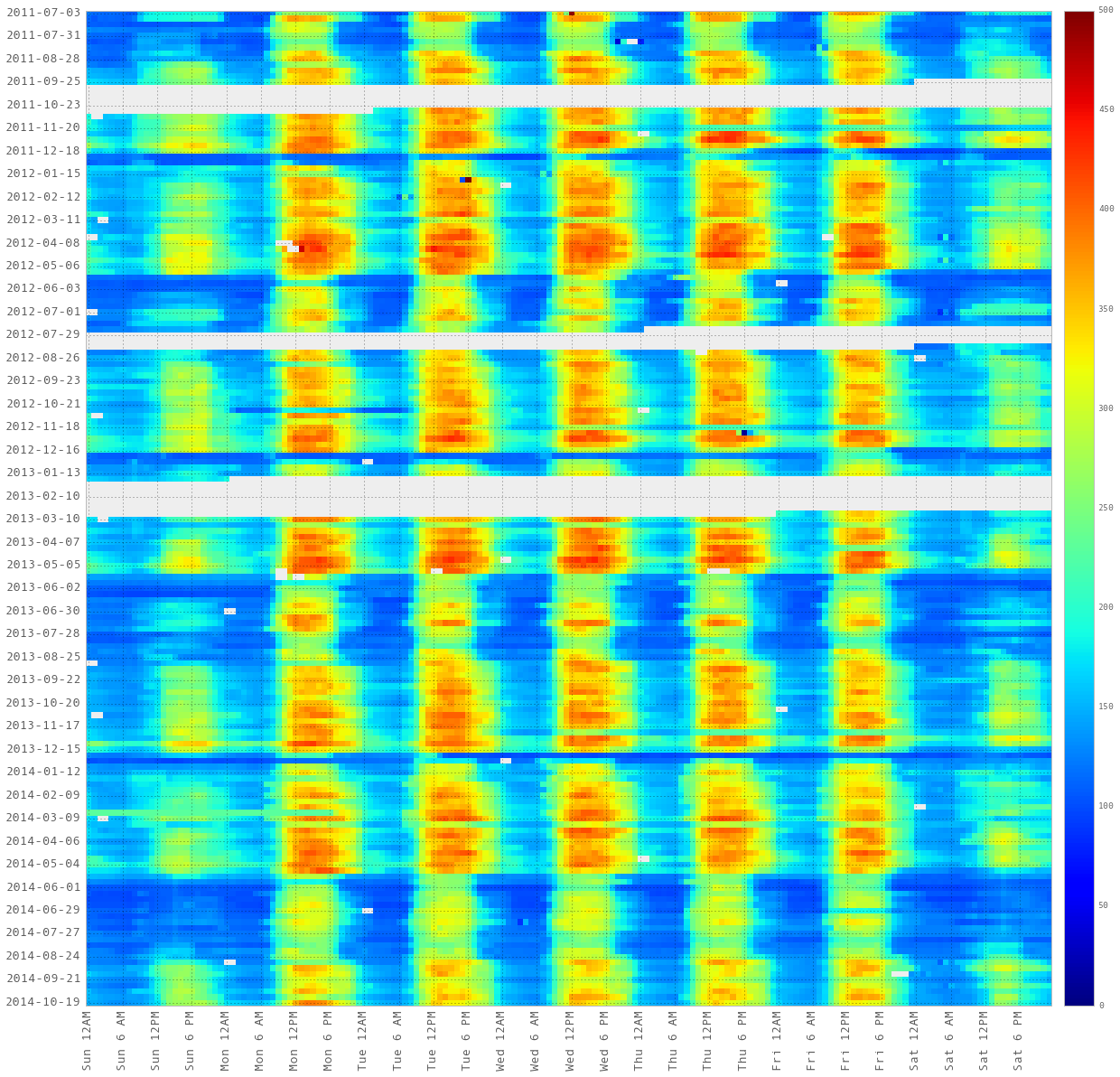
上图是三年内每小时用电量的累积图。banlk部分表示丢失的数据。
dailyElectricity = pd.read_excel('Data/dailyElectricity.xlsx')

index = (dailyElectricity['startDay'] >= np.datetime64('2011-07-03'))
	   &(dailyElectricity['startDay'] <  np.datetime64('2014-10-19'))
dailyElectricityForVisualization = dailyElectricity.loc[index,'electricity-kWh']

print "Data length: ", len(dailyElectricityForVisualization)/7, " weeks"

data = dailyElectricityForVisualization.values
data = data.reshape((len(data)/7/4,7*4))

from mpl_toolkits.axes_grid1 import make_axes_locatable

yTickLabels = pd.DataFrame(data = pd.date_range(start = '2011-07-03',
                                                end = '2014-10-25',
                                                freq = '4W',
                                                columns=['datetime'])
yTickLabels['date'] = yTickLabels['datetime'].apply(lambda x: x.strftime('%Y-%m-%d'))

s = ['Sun ', 'Mon ', 'Tue ', 'Wed ', 'Thu ', 'Fri ', 'Sat ']
xTickLabels = np.tile(s, 4)

fig = plt.figure(figsize=(14,15))
ax = plt.gca()
im = ax.imshow(data, interpolation='nearest', origin='upper')
divider = make_axes_locatable(ax)
cax = divider.append_axes("right", size="3%", pad=0.2)
ax.set_yticks(range(43))
ax.set_yticklabels(labels = yTickLabels['date'], fontsize = 14)

ax.set_xticks(range(28))
ax.set_xticklabels(labels = xTickLabels, fontsize = 14, rotation = 90)

plt.colorbar(im, cax=cax)
plt.show()

plt.figure()
fig = dailyElectricity.plot(figsize = (15, 6))
fig.set_axis_bgcolor('w')
plt.title('All the daily electricity data', fontsize = 16)
plt.ylabel('kWh')
plt.show()
Data length: 172.0 weeks

上面是一张热图和一张日常用电量图。空白部分表示缺少数据。
dailyElectricity = pd.read_excel('Data/dailyElectricity.xlsx')
weeklyElectricity = dailyElectricity.asfreq('W', how='sume', normalize=False)

plt.figure()
fig = weeklyElectricity['2012-01':'2014-01'].plot(figsize = (15, 6),
                                                  fontsize = 15,
                                                  marker = 'o',
                                                  linestyle='--')
fig.set_axis_bgcolor('w')
plt.title('Weekly electricity data', fontsize = 16)
plt.ylabel('kWh')
ax = plt.gca()
plt.show()

上面是每周消费的图表。折线部分表示数据丢失。
很明显,在决赛期间是最大的消耗。然后突然下降。重复的模式非常明显。
发现
-
电表现出强烈的周期性。你可以清楚地看到白天和晚上,工作日和周末的区别。
-
似乎在每个学期中,期末考试的用电量都会达到峰值,这可能代表了学习模式。学生们正越来越努力地准备期末考试。学期结束后会有一个假期,包括圣诞假期。1月和夏季学期的用电量相对较低,而春假期间校园可以相对空闲
能耗与特征的关系
我们考虑的主要特征
在这一节中,我们将电力、冷冻水和蒸汽消耗(每小时和每天)与各种特性进行对比。
# 从预处理结果中读取数据

hourlyElectricityWithFeatures =                            		pd.read_excel('Data/hourlyElectricityWithFeatures.xlsx')
hourlyChilledWaterWithFeatures = pd.read_excel('Data/hourlyChilledWaterWithFeatures.xlsx')
hourlySteamWithFeatures = pd.read_excel('Data/hourlySteamWithFeatures.xlsx')

dailyElectricityWithFeatures = pd.read_excel('Data/dailyElectricityWithFeatures.xlsx')
dailyChilledWaterWithFeatures = pd.read_excel('Data/dailyChilledWaterWithFeatures.xlsx')
dailySteamWithFeatures = pd.read_excel('Data/dailySteamWithFeatures.xlsx')

dailyChilledWaterWithFeatures.head()
| chilledWater-TonDays | startDay | endDay | RH-% | T-C | Tdew-C | pressure-mbar | solarRadiation-W/m2 | windDirection | windSpeed-m/s | humidityRatio-kg/kg | coolingDegrees | heatingDegrees | dehumidification | occupancy | |
|---|---|---|---|---|---|---|---|---|---|---|---|---|---|---|---|
| 2012-01-01 | 0.961857 | 2012-01-01 | 2012-01-02 | 76.652174 | 7.173913 | 3.073913 | 1004.956522 | 95.260870 | 236.086957 | 4.118361 | 0.004796 | 0 | 7.826087 | 0 | 0.0 |
| 2012-01-02 | 0.981725 | 2012-01-02 | 2012-01-03 | 55.958333 | 5.833333 | -2.937500 | 994.625000 | 87.333333 | 253.750000 | 5.914357 | 0.003415 | 0 | 9.166667 | 0 | 0.3 |
| 2012-01-03 | 1.003672 | 2012-01-03 | 2012-01-04 | 42.500000 | -3.208333 | -12.975000 | 1002.125000 | 95.708333 | 302.916667 | 6.250005 | 0.001327 | 0 | 18.208333 | 0 | 0.3 |
| 2012-01-04 | 1.483192 | 2012-01-04 | 2012-01-05 | 41.541667 | -7.083333 | -16.958333 | 1008.250000 | 98.750000 | 286.666667 | 5.127319 | 0.000890 | 0 | 22.083333 | 0 | 0.3 |
| 2012-01-05 | 3.465091 | 2012-01-05 | 2012-01-06 | 46.916667 | -0.583333 | -9.866667 | 1002.041667 | 90.750000 | 258.333333 | 5.162041 | 0.001746 | 0 | 15.583333 | 0 | 0.3 |
上面我们打印出所有的功能。
holidays = pd.read_excel('Data/holidays.xlsx')
holidays
| startDate | endDate | value | |
|---|---|---|---|
| 0 | 2011-07-01 | 2011-09-06 | 0.5 |
| 1 | 2011-10-10 | 2011-10-11 | 0.6 |
| 2 | 2011-11-24 | 2011-11-28 | 0.2 |
| 3 | 2011-12-22 | 2011-12-24 | 0.1 |
| 4 | 2011-12-24 | 2012-01-02 | 0.0 |
| 5 | 2012-01-02 | 2012-01-23 | 0.3 |
| 6 | 2012-03-10 | 2012-03-19 | 0.4 |
| 7 | 2012-05-17 | 2012-09-04 | 0.5 |
| 8 | 2012-05-28 | 2012-05-29 | 0.2 |
| 9 | 2012-10-08 | 2012-10-09 | 0.6 |
| 10 | 2012-11-22 | 2012-11-26 | 0.2 |
| 11 | 2012-12-22 | 2012-12-24 | 0.1 |
| 12 | 2012-12-24 | 2013-01-02 | 0.0 |
| 13 | 2013-01-02 | 2013-01-27 | 0.3 |
| 14 | 2013-01-20 | 2013-01-21 | 0.1 |
| 15 | 2013-03-16 | 2013-03-25 | 0.4 |
| 16 | 2013-05-18 | 2013-09-03 | 0.5 |
| 17 | 2013-10-14 | 2013-10-15 | 0.6 |
| 18 | 2013-11-28 | 2013-12-02 | 0.2 |
| 19 | 2013-12-20 | 2013-12-24 | 0.1 |
| 20 | 2013-12-24 | 2014-01-02 | 0.0 |
| 21 | 2014-01-02 | 2014-01-26 | 0.3 |
| 22 | 2014-03-16 | 2014-03-24 | 0.4 |
| 23 | 2014-05-17 | 2014-09-02 | 0.5 |
上面是“占用”的设置。全部入住率被赋值为1。
能源消耗与特征
fig, ax = plt.subplots(3, 2, sharey='row', figsize = (15, 12))
fig.subplots_adjust(hspace = 0.1, wspace = 0.1)

hourlyElectricityWithFeatures.plot(kind = 'scatter',
                                   x = 'T-C',
                                   y = 'electricity-kWh',
                                   ax = ax[0,0])
hourlyElectricityWithFeatures.plot(kind = 'scatter',
                                   x = 'coolingDegrees',
                                   y = 'electricity-kWh',
                                   ax = ax[0,1])
hourlyChilledWaterWithFeatures.plot(kind = 'scatter',
                                    x = 'T-C',
                                    y = 'chilledWater-TonDays',
                                    ax = ax[1,0])
hourlyChilledWaterWithFeatures.plot(kind = 'scatter',
                                    x = 'coolingDegrees',
                                    y = 'chilledWater-TonDays',
                                    ax = ax[1,1])
hourlySteamWithFeatures.plot(kind = 'scatter',
                             x = 'T-C',
                             y = 'steam-LBS',
                             ax = ax[2,0])
hourlySteamWithFeatures.plot(kind = 'scatter',
                             x = 'heatingDegrees',
                             y = 'steam-LBS',
                             ax = ax[2,1])

for i in range(3):
    ax[i,0].tick_params(which=u'major',
                        reset=False,
                        axis = 'y',
                        labelsize = 13)
    #ax[i,0].set_axis_bgcolor('w')

for i in range(2):
    ax[2,i].tick_params(which=u'major',
                        reset=False,
                        axis = 'x',
                        labelsize = 13)

ax[2,0].set_xlabel(r'Temperature ($^\circ$C)', fontsize = 13)
ax[2,0].set_xlim([-20,40])
ax[0,0].set_title(
    'Hourly energy use versus ourdoor temperature',
    fontsize = 15)

ax[2,1].set_xlabel(r'Cooling/Heating degrees ($^\circ$C)',
                   fontsize = 13)
#ax[2,1].set_xlim([0,30])
ax[0,1].set_title(
    'Hourly energy use versus cooling/heating degrees',
    fontsize = 15)

plt.show()

冷冻水和蒸汽与温度密切相关。然而,仅使用室外温度或冷却/加热温度来预测每小时的冷冻水和蒸汽是不够的。
fig, ax = plt.subplots(3, 2, sharey='row', figsize = (15, 12))
fig.subplots_adjust(hspace = 0.1, wspace = 0.1)

dailyElectricityWithFeatures.plot(kind = 'scatter',
                                  x = 'T-C',
                                  y = 'electricity-kWh',
                                  ax = ax[0,0])
dailyElectricityWithFeatures.plot(kind = 'scatter',
                                  x = 'coolingDegrees',
                                  y = 'electricity-kWh',
                                  ax = ax[0,1])
dailyChilledWaterWithFeatures.plot(kind = 'scatter',
                                   x = 'T-C',
                                   y = 'chilledWater-TonDays',
                                   ax = ax[1,0])
dailyChilledWaterWithFeatures.plot(kind = 'scatter',
                                   x = 'coolingDegrees',
                                   y = 'chilledWater-TonDays',
                                   ax = ax[1,1])
dailySteamWithFeatures.plot(kind = 'scatter',
                            x = 'T-C',
                            y = 'steam-LBS',
                            ax = ax[2,0])
dailySteamWithFeatures.plot(kind = 'scatter',
                            x = 'heatingDegrees',
                            y = 'steam-LBS',
                            ax = ax[2,1])

for i in range(3):
    ax[i,0].tick_params(which=u'major', reset=False, axis = 'y', labelsize = 13)
    #ax[i,0].set_axis_bgcolor('w')

for i in range(2):
    ax[2,i].tick_params(which=u'major', reset=False, axis = 'x', labelsize = 13)

ax[2,0].set_xlabel(r'Temperature ($^\circ$C)', fontsize = 13)
ax[2,0].set_xlim([-20,40])
ax[0,0].set_title('Daily energy use versus ourdoor temperature', fontsize = 15)

ax[2,1].set_xlabel(r'Cooling/Heating degrees ($^\circ$C)', fontsize = 13)
#ax[2,1].set_xlim([0,30])
ax[0,1].set_title('Daily energy use versus cooling/heating degrees', fontsize = 15)

plt.show()

日常冷冻水和蒸汽与室外温度有很强的线性关系。如果使用冷却/加热度而不是T-C,则应避免逐步线性回归。
fig, ax = plt.subplots(3, 2, sharex = 'col', sharey='row', figsize = (15, 12))
fig.subplots_adjust(hspace = 0.1, wspace = 0.1)

hourlyElectricityWithFeatures.plot(kind = 'scatter', x = 'humidityRatio-kg/kg', y = 'electricity-kWh', ax = ax[0,0])
hourlyElectricityWithFeatures.plot(kind = 'scatter', x = 'dehumidification', y = 'electricity-kWh', ax = ax[0,1])
hourlyChilledWaterWithFeatures.plot(kind = 'scatter', x = 'humidityRatio-kg/kg', y = 'chilledWater-TonDays', ax = ax[1,0])
hourlyChilledWaterWithFeatures.plot(kind = 'scatter', x = 'dehumidification', y = 'chilledWater-TonDays', ax = ax[1,1])
hourlySteamWithFeatures.plot(kind = 'scatter', x = 'humidityRatio-kg/kg', y = 'steam-LBS', ax = ax[2,0])
hourlySteamWithFeatures.plot(kind = 'scatter', x = 'dehumidification', y = 'steam-LBS', ax = ax[2,1])

for i in range(3):
    ax[i,0].tick_params(which=u'major', reset=False, axis = 'y', labelsize = 13)
    #ax[i,0].set_axis_bgcolor('w')

for i in range(2):
    ax[2,i].tick_params(which=u'major', reset=False, axis = 'x', labelsize = 13)

ax[2,0].set_xlabel(r'Humidity ratio (kg/kg)', fontsize = 13)
ax[2,0].set_xlim([0,0.02])
ax[0,0].set_title('Hourly energy use versus humidity ratio', fontsize = 15)

ax[2,1].set_xlabel(r'Dehumidification', fontsize = 13)
ax[2,1].set_xlim([0,0.01])
ax[0,1].set_title('Hourly energy use versus dehumidification', fontsize = 15)

plt.show()

湿度比肯定有助于预测冷冻水的消耗量,它优于RH和Tdrew。
fig, ax = plt.subplots(3, 2, sharex = 'col', sharey='row', figsize = (15, 12))
fig.subplots_adjust(hspace = 0.1, wspace = 0.1)

dailyElectricityWithFeatures.plot(kind = 'scatter',
                                  x = 'humidityRatio-kg/kg',
                                  y = 'electricity-kWh',
                                  ax = ax[0,0])
dailyElectricityWithFeatures.plot(kind = 'scatter',
                                  x = 'dehumidification',
                                  y = 'electricity-kWh',
                                  ax = ax[0,1])
dailyChilledWaterWithFeatures.plot(kind = 'scatter',
                                   x = 'humidityRatio-kg/kg',
                                   y = 'chilledWater-TonDays',
                                   ax = ax[1,0])
dailyChilledWaterWithFeatures.plot(kind = 'scatter',
                                   x = 'dehumidification',
                                   y = 'chilledWater-TonDays',
                                   ax = ax[1,1])
dailySteamWithFeatures.plot(kind = 'scatter',
                            x = 'humidityRatio-kg/kg',
                            y = 'steam-LBS',
                            ax = ax[2,0])
dailySteamWithFeatures.plot(kind = 'scatter',
                            x = 'dehumidification',
                            y = 'steam-LBS',
                            ax = ax[2,1])

for i in range(3):
    ax[i,0].tick_params(which=u'major', reset=False, axis = 'y', labelsize = 13)
    #ax[i,0].set_axis_bgcolor('w')

for i in range(2):
    ax[2,i].tick_params(which=u'major', reset=False, axis = 'x', labelsize = 13)

ax[2,0].set_xlabel(r'Humidity ratio (kg/kg)', fontsize = 13)
ax[2,0].set_xlim([0,0.02])
ax[0,0].set_title('Daily energy use versus humidity ratio', fontsize = 15)

ax[2,1].set_xlabel(r'Dehumidification', fontsize = 13)
ax[2,1].set_xlim([0,0.01])
ax[0,1].set_title('Daily energy use versus dehumidification', fontsize = 15)

plt.show()
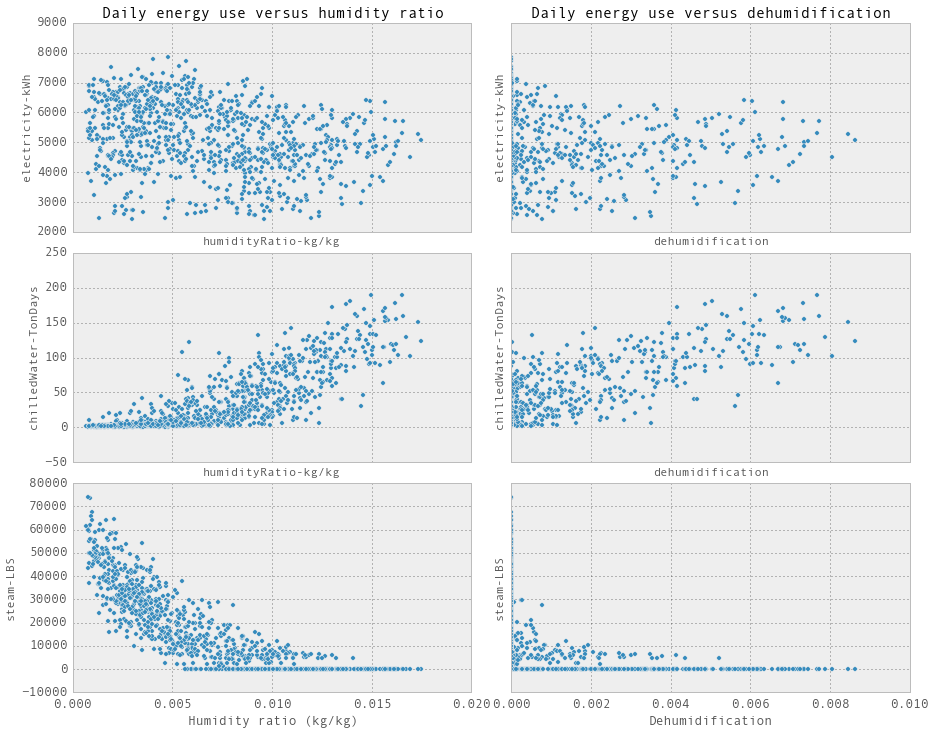
除湿是用来预测冷水的,而不是蒸汽。
fig, ax = plt.subplots(3, 2, sharex = 'col', figsize = (15, 12))
fig.subplots_adjust(hspace = 0.1, wspace = 0.15)

hourlyElectricityWithFeatures.plot(kind = 'scatter',
                                   x = 'occupancy',
                                   y = 'electricity-kWh',
                                   ax = ax[0,0])
dailyElectricityWithFeatures.plot(kind = 'scatter',
                                  x = 'occupancy',
                                  y = 'electricity-kWh',
                                  ax = ax[0,1])
hourlyChilledWaterWithFeatures.plot(kind = 'scatter',
                                    x = 'occupancy',
                                    y = 'chilledWater-TonDays',
                                    ax = ax[1,0])
dailyChilledWaterWithFeatures.plot(kind = 'scatter',
                                   x = 'occupancy',
                                   y = 'chilledWater-TonDays',
                                   ax = ax[1,1])
hourlySteamWithFeatures.plot(kind = 'scatter',
                             x = 'occupancy',
                             y = 'steam-LBS',
                             ax = ax[2,0])
dailySteamWithFeatures.plot(kind = 'scatter',
                            x = 'occupancy',
                            y = 'steam-LBS',
                            ax = ax[2,1])

for i in range(3):
    ax[i,0].tick_params(which=u'major', reset=False, axis = 'y', labelsize = 13)
    #ax[i,0].set_axis_bgcolor('w')

for i in range(2):
    ax[2,i].tick_params(which=u'major', reset=False, axis = 'x', labelsize = 13)

ax[2,0].set_xlabel(r'Occupancy', fontsize = 13)
#ax[2,0].set_xlim([0,0.02])
ax[0,0].set_title('Hourly energy use versus occupancy', fontsize = 15)

ax[2,1].set_xlabel(r'Occupancy', fontsize = 13)

#ax[2,1].set_xlim([0,0.01])
ax[0,1].set_title('Daily energy use versus occupancy', fontsize = 15)

plt.show()

入住率来源于学年、假期和周末。基本上,我们只是给假期、周末和夏天赋了一个较低的值。cosHour,入住率可能有用,也可能没用,因为它们只是对入住率的估计。
fig, ax = plt.subplots(3, 1, sharex = 'col', figsize = (8, 12))
fig.subplots_adjust(hspace = 0.1, wspace = 0.15)

hourlyElectricityWithFeatures.plot(kind = 'scatter',
                                   x = 'cosHour',
                                   y = 'electricity-kWh',
                                   ax = ax[0])
hourlyChilledWaterWithFeatures.plot(kind = 'scatter',
                                    x = 'cosHour',
                                    y = 'chilledWater-TonDays',
                                    ax = ax[1])
hourlySteamWithFeatures.plot(kind = 'scatter',
                             x = 'cosHour',
                             y = 'steam-LBS',
                             ax = ax[2])

for i in range(3):
    ax[i].tick_params(which=u'major', reset=False, axis = 'y', labelsize = 13)
    #ax[i,0].set_axis_bgcolor('w')

ax[2].tick_params(which=u'major', reset=False, axis = 'x', labelsize = 13)

ax[2].set_xlabel(r'cosHour', fontsize = 13)
#ax[2,0].set_xlim([0,0.02])
ax[0].set_title('Hourly energy use versus cosHourOfDay', fontsize = 15)

plt.show()

能源利用与cosHour之间存在一定的联系.
fig, ax = plt.subplots(3, 2, sharex = 'col', sharey = 'row', figsize = (15, 12))
fig.subplots_adjust(hspace = 0.1, wspace = 0.15)
hourlyElectricityWithFeatures.plot(kind = 'scatter',
x = 'solarRadiation-W/m2',
y = 'electricity-kWh',
ax = ax[0,0])
hourlyElectricityWithFeatures.plot(kind = 'scatter',
x = 'windSpeed-m/s',
y = 'electricity-kWh',
ax = ax[0,1])
hourlyChilledWaterWithFeatures.plot(kind = 'scatter',
x = 'solarRadiation-W/m2',
y = 'chilledWater-TonDays',
ax = ax[1,0])
hourlyChilledWaterWithFeatures.plot(kind = 'scatter',
x = 'windSpeed-m/s',
y = 'chilledWater-TonDays',
ax = ax[1,1])
hourlySteamWithFeatures.plot(kind = 'scatter',
x = 'solarRadiation-W/m2',
y = 'steam-LBS',
ax = ax[2,0])
hourlySteamWithFeatures.plot(kind = 'scatter',
x = 'windSpeed-m/s',
y = 'steam-LBS',
ax = ax[2,1])
for i in range(3):
ax[i,0].tick_params(which=u'major', reset=False, axis = 'y', labelsize = 13)
#ax[i,0].set_axis_bgcolor('w')
for i in range(2):
ax[2,i].tick_params(which=u'major', reset=False, axis = 'x', labelsize = 13)
ax[2,0].set_xlabel(r'Solar radiation (W/m2)', fontsize = 13)
#ax[2,0].set_xlim([0,0.02])
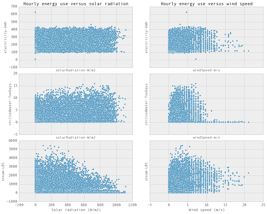
ax[0,0].set_title('Hourly energy use versus solar radiation', fontsize = 15)
ax[2,1].set_xlabel(r'Wind speed (m/s)', fontsize = 13)
#ax[2,1].set_xlim([0,0.01])
ax[0,1].set_title('Hourly energy use versus wind speed', fontsize = 15)
plt.show()
fig, ax = plt.subplots(3, 2, sharex = 'col', sharey = 'row', figsize = (15, 12))
fig.subplots_adjust(hspace = 0.1, wspace = 0.15)

dailyElectricityWithFeatures.plot(kind = 'scatter',
                                  x = 'solarRadiation-W/m2',
                                  y = 'electricity-kWh',
                                  ax = ax[0,0])
dailyElectricityWithFeatures.plot(kind = 'scatter',
                                  x = 'windSpeed-m/s',
                                  y = 'electricity-kWh',
                                  ax = ax[0,1])
dailyChilledWaterWithFeatures.plot(kind = 'scatter',
                                   x = 'solarRadiation-W/m2',
                                   y = 'chilledWater-TonDays',
                                   ax = ax[1,0])
dailyChilledWaterWithFeatures.plot(kind = 'scatter',
                                   x = 'windSpeed-m/s',
                                   y = 'chilledWater-TonDays',
                                   ax = ax[1,1])
dailySteamWithFeatures.plot(kind = 'scatter',
                            x = 'solarRadiation-W/m2',
                            y = 'steam-LBS',
                            ax = ax[2,0])
dailySteamWithFeatures.plot(kind = 'scatter',
                            x = 'windSpeed-m/s',
                            y = 'steam-LBS',
                            ax = ax[2,1])

for i in range(3):
    ax[i,0].tick_params(which=u'major', reset=False, axis = 'y', labelsize = 13)
    #ax[i,0].set_axis_bgcolor('w')

for i in range(2):
    ax[2,i].tick_params(which=u'major', reset=False, axis = 'x', labelsize = 13)

ax[2,0].set_xlabel(r'Solar radiation (W/m2)', fontsize = 13)
#ax[2,0].set_xlim([0,0.02])
ax[0,0].set_title('Daily energy use versus solar radiation', fontsize = 15)

ax[2,1].set_xlabel(r'Wind speed (m/s)', fontsize = 13)

#ax[2,1].set_xlim([0,0.01])
ax[0,1].set_title('DAily energy use versus wind speed', fontsize = 15)

plt.show()
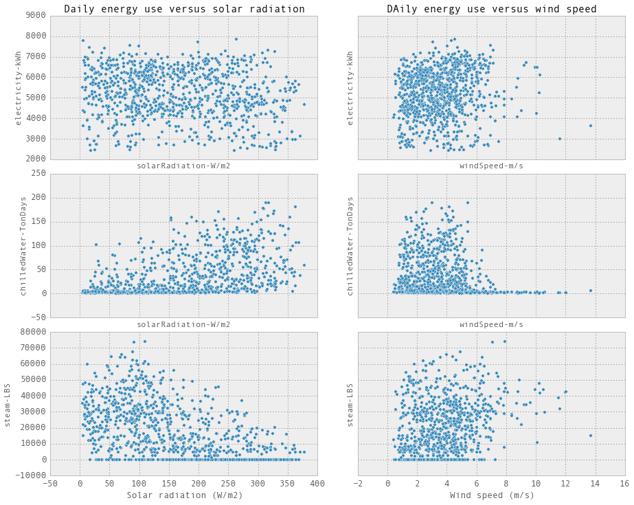
太阳辐射和风速并不那么重要,它们与温度有关。
发现
-
电力与天气数据(温度)无关。利用天气信息来预测电力的想法是行不通的。我认为这主要取决于时间/入住率。但是我们仍然可以做一些模式探索来找出白天/晚上、工作日/周末、学校日/假期的用电模式。实际上,我们应该从月度数据中注意到这一点。
-
冷冻水和蒸汽与温度和湿度密切相关。日冷水、蒸汽消耗量与冷热度呈良好的线性关系。因此,简单的线性回归可能已经足够精确了。
-
虽然冷水和热水的消耗与天气有很强的相关性,但是根据上面的图用天气信息来预测每小时的冷冻水和蒸汽是不够的。这是因为运行计划影响每小时的能源消耗。每小时的冷水和蒸汽预测必须包括用房和运行计划。
-
湿度比肯定有助于预测冷水的消耗量,它优于RH和Tdrew。
-
冷和热温度将有助于预测每天的冷冻水和蒸汽。如果使用冷却/加热度而不是T-C,则应避免逐步线性回归。
-
入住率来源于学年、假期和周末。基本上,我们只是给假期、周末和夏天赋了一个较低的值。cosHour,入住率可能有用,也可能没用,因为它们只是对入住率的估计。

 浙公网安备 33010602011771号