
python库skimage 对图像进行gamma校正和log校正
Gamma校正
Gamma校正是对输入图像灰度值进行的非线性操作,使输出图像灰度值与输入图像灰度值呈指数关系:
这个指数即为Gamma。
Gamma校正的原理很简单,就一个很简单的表达式,如下图所示:
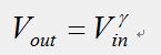
其中V_in的取值范围是0~1,最重要的参数就是公式中的γ参数!
γ的值决定了输入图像和输出图像之间的灰度映射方式,即决定了是增强低灰度值区域还是增高灰度值区域。
γ>1时,图像的高灰度区域对比度得到增强。
γ<1时,图像的低灰度区域对比度得到增强。
γ=1时,不改变原图像。
伽马变换对于图像对比度偏低,并且整体亮度值偏高(对于于相机过曝)情况下的图像增强效果明显。
对数log变换
log 函数的表达式:
y=alog(1+x), a 是一个放大系数,x 同样是输入的像素值,取值范围为 [0−1], y 是输出的像素值。
对数变换对于整体对比度偏低并且灰度值偏低的图像增强效果较好。
skimage库实现gamam校正和log校正
函数:
Gamma:
gamma_corrected = exposure.adjust_gamma(img, 2)
Logarithmic:
logarithmic_corrected = exposure.adjust_log(img, 1)
"""
=================================
Gamma and log contrast adjustment
=================================

This example adjusts image contrast by performing a Gamma and a Logarithmic
correction on the input image.

"""
import matplotlib
import matplotlib.pyplot as plt
import numpy as np

from skimage import data, img_as_float
from skimage import exposure

matplotlib.rcParams['font.size'] = 8


def plot_img_and_hist(image, axes, bins=256):
    """Plot an image along with its histogram and cumulative histogram.

    """
    image = img_as_float(image)
    ax_img, ax_hist = axes
    ax_cdf = ax_hist.twinx()

    # Display image
    ax_img.imshow(image, cmap=plt.cm.gray)
    ax_img.set_axis_off()

    # Display histogram
    ax_hist.hist(image.ravel(), bins=bins, histtype='step', color='black')
    ax_hist.ticklabel_format(axis='y', style='scientific', scilimits=(0, 0))
    ax_hist.set_xlabel('Pixel intensity')
    ax_hist.set_xlim(0, 1)
    ax_hist.set_yticks([])

    # Display cumulative distribution
    img_cdf, bins = exposure.cumulative_distribution(image, bins)
    ax_cdf.plot(bins, img_cdf, 'r')
    ax_cdf.set_yticks([])

    return ax_img, ax_hist, ax_cdf


# Load an example image
img = data.moon()

# Gamma
gamma_corrected = exposure.adjust_gamma(img, 2)

# Logarithmic
logarithmic_corrected = exposure.adjust_log(img, 1)

# Display results
fig = plt.figure(figsize=(8, 5))
axes = np.zeros((2, 3), dtype=np.object)
axes[0, 0] = plt.subplot(2, 3, 1)
axes[0, 1] = plt.subplot(2, 3, 2, sharex=axes[0, 0], sharey=axes[0, 0])
axes[0, 2] = plt.subplot(2, 3, 3, sharex=axes[0, 0], sharey=axes[0, 0])
axes[1, 0] = plt.subplot(2, 3, 4)
axes[1, 1] = plt.subplot(2, 3, 5)
axes[1, 2] = plt.subplot(2, 3, 6)

ax_img, ax_hist, ax_cdf = plot_img_and_hist(img, axes[:, 0])
ax_img.set_title('Low contrast image')

y_min, y_max = ax_hist.get_ylim()
ax_hist.set_ylabel('Number of pixels')
ax_hist.set_yticks(np.linspace(0, y_max, 5))

ax_img, ax_hist, ax_cdf = plot_img_and_hist(gamma_corrected, axes[:, 1])
ax_img.set_title('Gamma correction')

ax_img, ax_hist, ax_cdf = plot_img_and_hist(logarithmic_corrected, axes[:, 2])
ax_img.set_title('Logarithmic correction')

ax_cdf.set_ylabel('Fraction of total intensity')
ax_cdf.set_yticks(np.linspace(0, 1, 5))

# prevent overlap of y-axis labels
fig.tight_layout()
plt.show()
实验结果


 浙公网安备 33010602011771号