
深入解析:Deep Learning|02 Handcraft Code of BRF Network
Deep Learning|02 Handcraft Code of BRF Network
Implement a RBF Network in Stock
文章目录
Genrally, training RBF network is divided into two steps: the first step is to select the centers of neurons; the second step is to optimize the network parameters using the BP algorithm. There are many methods for selecting neuron centers, such as random selection, clustering-based selection, and so on. At the same time, we can also select the centers of RBFs through supervised learning, which is also the most general form of RBF networks.
Based on RBF general form, mathmatical training process of RBF network!
We will derive the training process of RBF network based on Gauss core.
1. Gauss core
The definition of Gauss core is :
Φ ( x i , c j ) = e − ∥ x i − c j ∥ 2 2 σ 2 \begin{align*} \Phi(x_i, c_j) = e^{-\frac{\|x_i - c_j\|^2}{2\sigma^2}} \end{align*}Φ(xi,cj)=e−2σ2∥xi−cj∥2
where c j c_jcjis the center point of thej jj-th neuron;σ \sigmaσis the width of the Gaussian kernel, and∥ x i − c j ∥ \|x_i - c_j\|∥xi−cj∥is the Euclidean distance from the samplex i x_ixito the center pointc j c_jcj.
2. BRF network
BRF network is defined by :
f ( x ) = ∑ j = 1 q w j ⋅ Φ ( x , c j ) f(x) = \sum_{j=1}^{q} w_j \cdot \Phi(x, c_j)f(x)=j=1∑qwj⋅Φ(x,cj)
where w j w_jwjis theweightof thej jj-th neuron,q qqis the total number of neuron.
3. Error function
We define the error function as the mean squared error, and the goal is to minimize the error function:
E = 1 2 m ∑ i = 1 m e i 2 = 1 2 m ∑ i = 1 m ( f ( x ) − y ) 2 = 1 2 m ∑ i = 1 m ( ∑ j = 1 q w j ⋅ Φ ( x , c j ) − y ) 2 \begin{align*} E &= \frac{1}{2m} \sum_{i=1}^{m} e_i^2 \\ &= \frac{1}{2m} \sum_{i=1}^{m} (f(x) - y)^2 \\&= \frac{1}{2m} \sum_{i=1}^{m} \left( \sum_{j=1}^{q} w_j \cdot \Phi(x, c_j) - y \right)^2 \end{align*}E=2m1i=1∑mei2=2m1i=1∑m(f(x)−y)2=2m1i=1∑m(j=1∑qwj⋅Φ(x,cj)−y)2
We use the BP algorithm to propagate errors backward and the Gradient Descent method to respectively determine the optimization directions for the parameters of the RBF network.
Linear weights of output layer neurons
Δ w = ∂ E ∂ w = 1 m ∑ i = 1 m ( f ( x ) − y ) ⋅ φ ( x , c ) = 1 m ∑ i = 1 m e i ⋅ φ ( x , c ) \Delta w = \frac{\partial E}{\partial w} = \frac{1}{m} \sum_{i=1}^{m} (f(x) - y) \cdot \varphi(x, c) = \frac{1}{m} \sum_{i=1}^{m} e_i \cdot \varphi(x, c)Δw=∂w∂E=m1i=1∑m(f(x)−y)⋅φ(x,c)=m1i=1∑mei⋅φ(x,c)Weight iteration formula
w k + 1 = w k − η ⋅ Δ w w_{k+1} = w_k - \eta \cdot \Delta wwk+1=wk−η⋅Δw
- Neuron center points of hidden layer
Δ c j = ∂ E ∂ c j = ∂ E ∂ φ ( x , c j ) ⋅ ∂ φ ( x , c j ) ∂ c j = 1 m ∑ i = 1 m ( f ( x ) − y ) w ⋅ ∂ φ ( x , c j ) ∂ c j = 1 m ∑ i = 1 m ( f ( x ) − y ) w ⋅ φ ( x , c j ) ⋅ x − c j σ j 2 = 1 m ⋅ σ j 2 ∑ i = 1 m ( f ( x ) − y ) w ⋅ φ ( x , c j ) ⋅ ( x − c j ) \begin{aligned} \Delta c_j &= \frac{\partial E}{\partial c_j} = \frac{\partial E}{\partial \varphi(x, c_j)} \cdot \frac{\partial \varphi(x, c_j)}{\partial c_j} \\ &= \frac{1}{m} \sum_{i=1}^{m} (f(x) - y) w \cdot \frac{\partial \varphi(x, c_j)}{\partial c_j} \\ &= \frac{1}{m} \sum_{i=1}^{m} (f(x) - y) w \cdot \varphi(x, c_j) \cdot \frac{x - c_j}{\sigma_j^2} \\ &= \frac{1}{m \cdot \sigma_j^2} \sum_{i=1}^{m} (f(x) - y) w \cdot \varphi(x, c_j) \cdot (x - c_j) \end{aligned}Δcj=∂cj∂E=∂φ(x,cj)∂E⋅∂cj∂φ(x,cj)=m1i=1∑m(f(x)−y)w⋅∂cj∂φ(x,cj)=m1i=1∑m(f(x)−y)w⋅φ(x,cj)⋅σj2x−cj=m⋅σj21i=1∑m(f(x)−y)w⋅φ(x,cj)⋅(x−cj)
Neuron center point iteration formula
c k + 1 = c k − η ⋅ Δ c c_{k+1} = c_k - \eta \cdot \Delta cck+1=ck−η⋅Δc
- Gaussian kernel width of hidden layer
Δ σ j = ∂ E ∂ σ j = ∂ E ∂ φ ( x , c j ) ⋅ ∂ Φ ( x , c j ) ∂ σ j = 1 m ∑ i = 1 m ( f ( x ) − y ) w ⋅ ∂ Φ ( x , c j ) ∂ σ j = 1 m ⋅ σ j 3 ∑ i = 1 m ( f ( x ) − y ) w ⋅ Φ ( x , c j ) ⋅ ∥ x i − c j ∥ 2 \begin{aligned} \Delta \sigma_j &= \frac{\partial E}{\partial \sigma_j} = \frac{\partial E}{\partial \varphi(x, c_j)} \cdot \frac{\partial \Phi(x, c_j)}{\partial \sigma_j} \\ &= \frac{1}{m} \sum_{i=1}^{m} (f(x) - y) w \cdot \frac{\partial \Phi(x, c_j)}{\partial \sigma_j} \\ &= \frac{1}{m \cdot \sigma_j^3} \sum_{i=1}^{m} (f(x) - y) w \cdot \Phi(x, c_j) \cdot \| x_i - c_j \|^2 \end{aligned}Δσj=∂σj∂E=∂φ(x,cj)∂E⋅∂σj∂Φ(x,cj)=m1i=1∑m(f(x)−y)w⋅∂σj∂Φ(x,cj)=m⋅σj31i=1∑m(f(x)−y)w⋅Φ(x,cj)⋅∥xi−cj∥2
Gaussian kernel width iteration formula
σ
k
+
1
=
σ
k
−
η
⋅
Δ
σ
\sigma_{k+1} = \sigma_k - \eta \cdot \Delta \sigmaσk+1=σk−η⋅Δσ
Handcraft code
import numpy as np
import matplotlib.pyplot as plt
import os
class BRF:
def __init__(self, hidden_nums, r_w, r_c, r_sigma, tol=1e-5):
self.hidden_nums = hidden_nums
self.r = {
'w': r_w,
'c': r_c,
'sigma': r_sigma
}
self.tol = tol
self.errList = []
self.c = None
self.w = None
self.sigma = None
def train(self, X, y, iters):
self.X = X
self.y = y.reshape(-1, 1)
self.n_samples, self.n_features = X.shape
sigma, c, w = self.init()
for i in range(iters):
hi_output = self.change(sigma, X, c)
yi_input = self.addIntercept(hi_output)
yi_output = np.dot(yi_input, w)
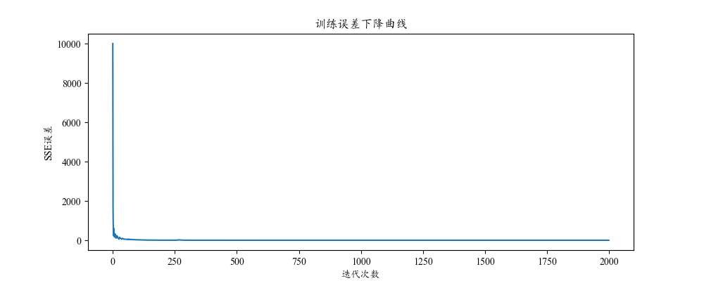
error = self.calSSE(yi_output, self.y)
if error < self.tol:
break
self.errList.append(error)
delta_w = np.dot(yi_input.T, (yi_output - self.y))
w -= self.r['w'] * delta_w / self.n_samples
delta_sigma = np.divide(
np.multiply(
np.dot(np.multiply(hi_output, self.l2(X, c)).T, (yi_output - self.y)),
w[:-1]
),
sigma**3
)
sigma -= self.r['sigma'] * delta_sigma / self.n_samples
deltac1 = np.divide(w[:-1], sigma**2)
deltac2 = np.zeros((1, self.n_features))
for j in range(self.n_samples):
deltac2 += (yi_output - self.y)[j] * np.dot(hi_output[j], X[j] - c)
deltac = np.dot(deltac1, deltac2)
c -= self.r['c'] * deltac / self.n_samples
self.c = c
self.w = w
self.sigma = sigma
self.n_iters = i
def guass(self, sigma, X, ci):
return np.exp(-np.linalg.norm((X - ci), axis=1)**2 / (2 * sigma**2))
def change(self, sigma, X, c):
newX = np.zeros((self.n_samples, len(c)))
for i in range(len(c)):
newX[:, i] = self.guass(sigma[i], X, c[i])
return newX
def init(self):
sigma = np.random.random((self.hidden_nums, 1))
c = np.random.random((self.hidden_nums, self.n_features))
w = np.random.random((self.hidden_nums + 1, 1))
return sigma, c, w
def addIntercept(self, X):
return np.hstack((X, np.ones((self.n_samples, 1))))
def calSSE(self, prey, y):
return 0.5 * (np.linalg.norm(prey - y))**2
def l2(self, X, c):
m, n = np.shape(X)
newX = np.zeros((m, len(c)))
for i in range(len(c)):
newX[:, i] = np.linalg.norm((X - c[i]), axis=1)**2
return newX
def predict(self, X):
hi_output = self.change(self.sigma, X, self.c)
yi_input = self.addIntercept(hi_output)
yi_output = np.dot(yi_input, self.w)
return yi_output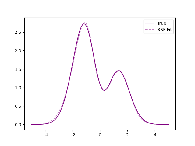


 浙公网安备 33010602011771号