06 Logistic Regression

回归与分类

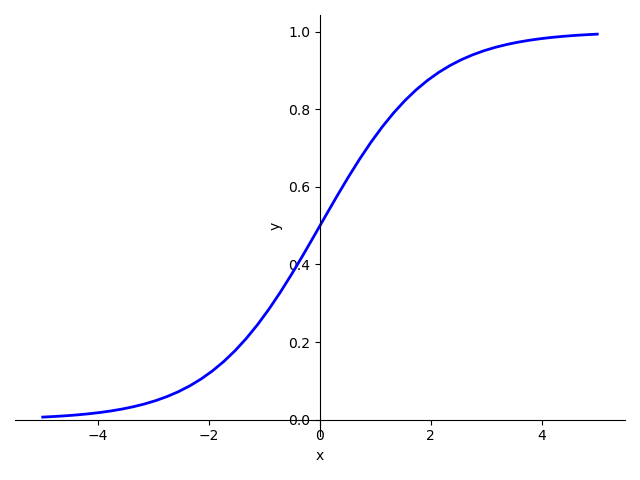
1. 回归->分类：将实数空间\(R\)映射到\([0,1]\)
2. Logistic函数\(y=\frac{1}{1+e^{-x}}\)
   

损失函数

线性回归的损失函数

\[loss\ =\ (\hat{y}-y)^{2}=(x*\omega-y)^{2} \]

二分类的损失函数(交叉熵)

\[loss\ =\ -(ylog\hat{y}+(1-y)log(1-\hat{y})) \]

Mini-Batch损失函数

对二分类的损失函数求均值

\[loss\ =\ -\frac{1}{N}\sum_{n=1}^N(y_{n}log\hat{y_n}+(1-y_{n}log(1-\hat{y_n}))) \]

与线性回归的区别

1. 在前馈中多了一个sigmoid的处理
2. 损失函数不再是MSELoss，而是BSELoss以求交叉熵

代码实现

训练数据是x表示学习时间，y表示是否合格（0不合格，1合格）

from abc import ABC
import torch
import matplotlib.pyplot as plt

x_data = torch.Tensor([[1.0], [2.0], [3.0]])
y_data = torch.Tensor([[0], [0], [1]])


class LogisticRegressionModel(torch.nn.Module, ABC):
    def __init__(self):
        super(LogisticRegressionModel, self).__init__()
        self.linear = torch.nn.Linear(1, 1)

    def forward(self, x):
        y_pred = torch.sigmoid(self.linear(x))
        return y_pred


model = LogisticRegressionModel()

criterion = torch.nn.BCELoss(size_average=False)
optimizer = torch.optim.SGD(model.parameters(), lr=0.01)

loss_list = []
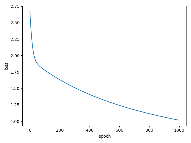
for epoch in range(1000):
    y_pred = model(x_data)
    loss = criterion(y_pred, y_data)
    print(epoch, loss.item())

    loss_list.append(loss.item())
    optimizer.zero_grad()
    loss.backward()
    optimizer.step()

epoch_list = list(range(1000))
plt.plot(epoch_list, loss_list)
plt.xlabel("epoch")
plt.ylabel("loss")
plt.show()

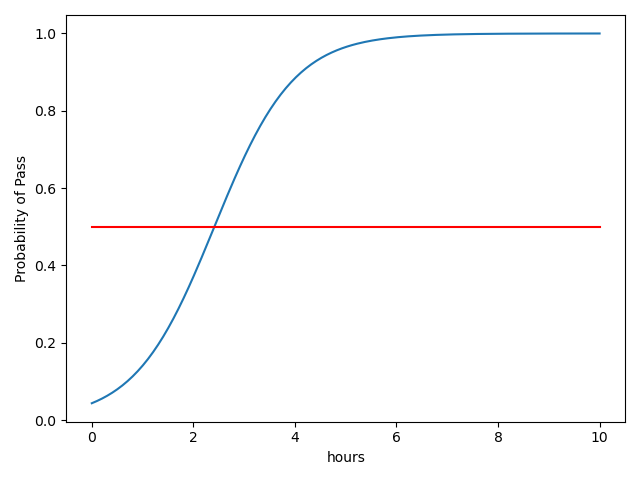
测试

import numpy as np
import matplotlib.pyplot as plt

x = np.linspace(0, 10, 200)
x_test = torch.Tensor(x).view(200, 1) # reshape 200行 1列
y_test = model(x_test)
y = y_test.data.numpy()
plt.plot(x, y)
plt.plot([0, 10], [0.5, 0.5], c='r')
plt.xlabel("hours")
plt.ylabel('Probability of Pass')
plt.show()

Reference

https://www.bilibili.com/video/BV1Y7411d7Ys?p=6