[CS231n]SVM and Softmax

[CS231n]SVM and Softmax

回顾

上一讲是\(KNN\)算法，是惰性算法，他不需要显示的构建模型，抽取特征，他只是在构建的时候需要找到那个就去找到跟他最近邻的数据，基本不需要训练，但是预测的时候是很慢的。\(Train~O(1),Predict~O(n)\) 随着样本增加，其复杂度是线性增加的，但是随着维度的增加，其样本数是呈指数爆炸增长的，\(KNN\)算法的性能是比较差的。在训练集较少的情况下可以使用交叉验证方法来选取\(K\),来尽可能减少偶然误差，评估模型的性能。

SVM

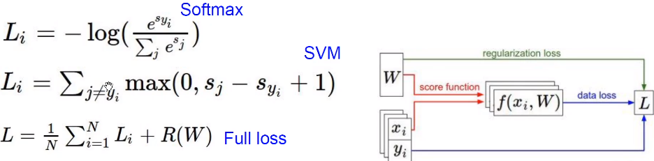
损失函数：说明了目前这个分类器的工作情况

我们设有 \(x_i~s~image~and~y_i~s(integer)~label\) 则有

\[L=\frac{1}{N}\sum L_i(f(x_i,W),y_i) \]

这里\(f(x_i,W),y_i\) 就是把分数和每一个具体的标签进行比较，然后对所有的损失函数值取平均值。

Hinge loss

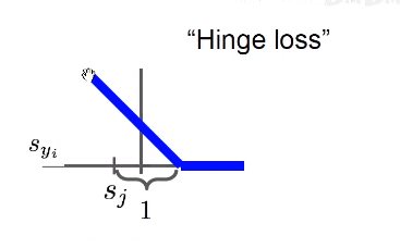
\[L_i=\begin{cases} 0~~~~~~~~~~~~~~~~~~~if~s_{y_i}>=S_j+1\newline s_j-s_i+1~~otherwise \end{cases} \]

Eg:

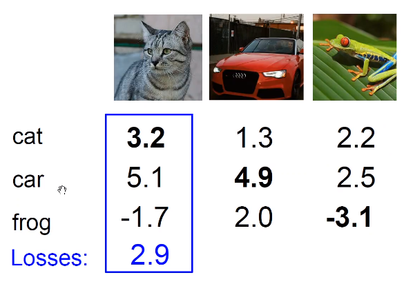
这里对于猫的计算是\(max(0,5.1-3.2+1)+max(0,-1.7-3.2+1)=2.9\)

这里并没有对自生做这个计算，( 实际上，就算对自生做这个处理，也只是，对每一项的 loss加上了 1，并不会影响最终的结果，因为我们在这里看的是二者相对的值。)铰链损失函数会惩罚分数差1以上的项目，对于其他不进行惩罚。

Q1：如果汽车的分值发生了一点的变化？

并不会改变，因为1这个值的存在。

实际上1这个值是有讲究的，我们并不关心这个值的绝对的大小，而是相对的大小，1其实是单位1的意思。

Q2:最小、最大值是多少？

0-正无穷

Q3:在一开始\(W\)很小所以\(s->0\)那么\(loss\)值是多少？

应该是分类错误的类别的个数

Q4:在计算的时候加上了计算正确的类别？ 同上正文所讲

Q5:如果平均而不是求和？ 只是改了一个常数无影响

Q6:使用了平方损失函数？ 惩罚项被放大了

def L_i_vectorized(x, y, w):
    scores = W.dot(x)
    margins = sp.maximum(0, scores - scores[y] + 1)
    margins[y] = 0  # 这里是因为在上一步其把自身也减去了
    loss_i = np.sum(margins)
    return loss_i

如果\(loss=0\):

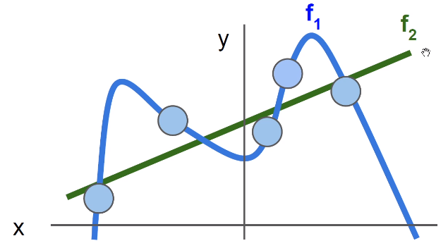
同一个损失函数可以对应于很多个不同的\(W\)，这里引入正则化，防止过拟合。

\[L=\frac{1}{N}\sum L_i(f(x_i,W),y_i)+\lambda R(W) \]

\[\text{L2 regularization:}R(W)=\sum_k \sum_l W_{k,l}^2 \]

\[\text{L1 regularization:}R(W)=\sum_k \sum_l |W_{k,l}| \]

\[\text{Elastic net(L1+L2):}R(W)=\sum_k \sum_l \beta W_{k,l}^2 +|W_{k,l}| \]

正则化让模型更加简单(drop out,batch normalization……)，让其在测试集上可以更好的泛化。显然下图\(f_2\)更加好

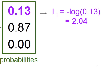
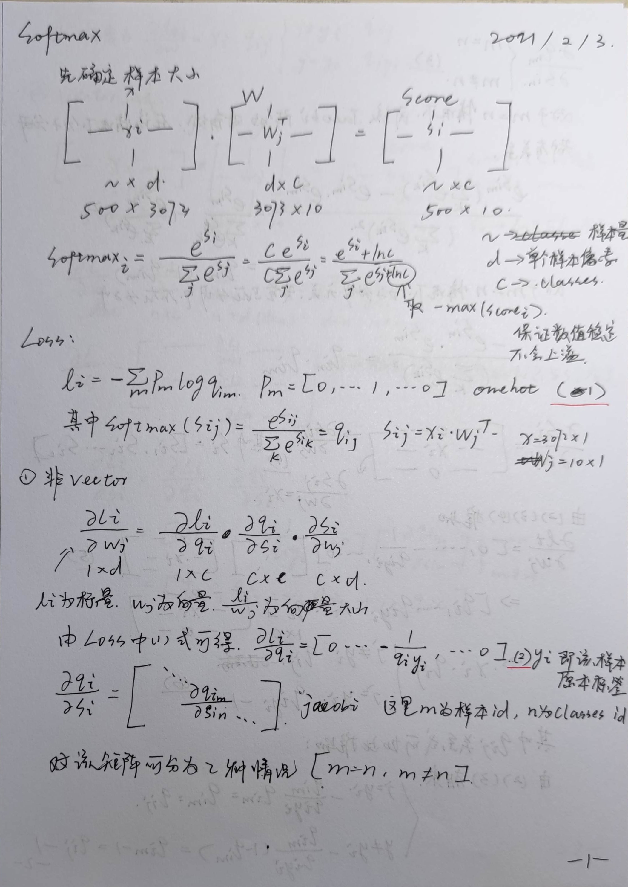
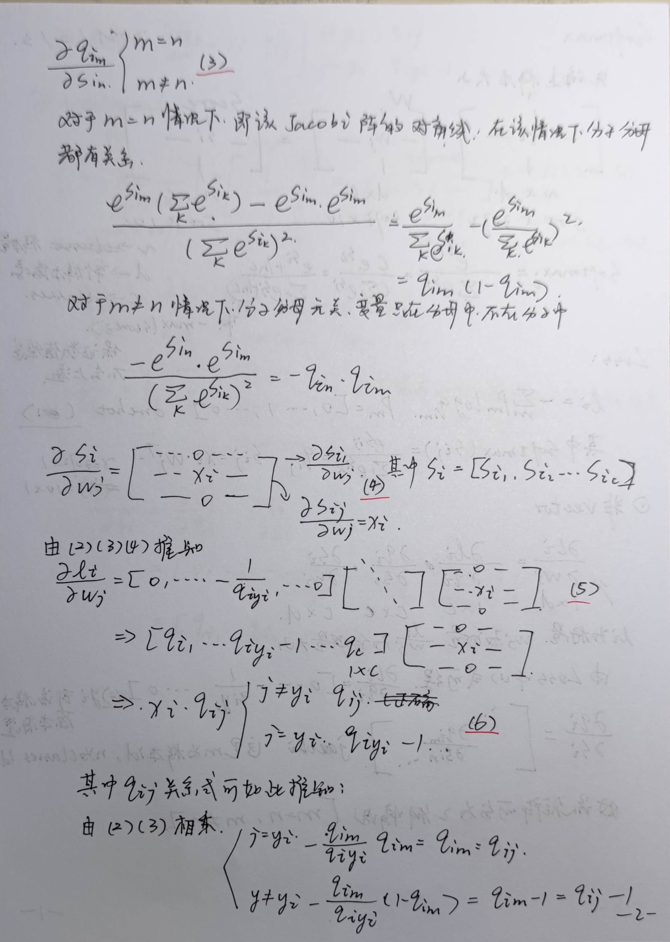
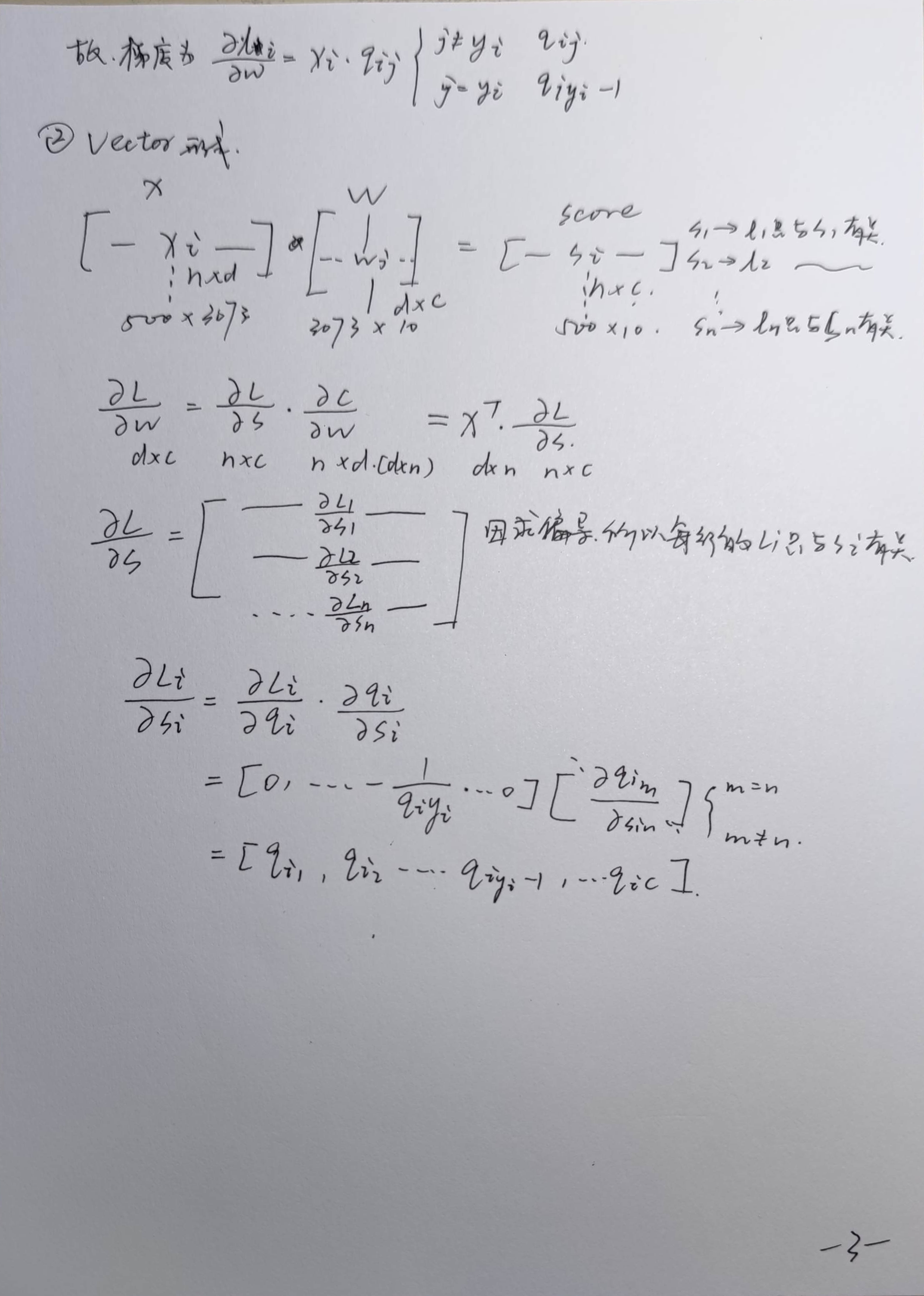
Softmax Classifier

先用指数函数的形式变成正数，接下来归一化处理

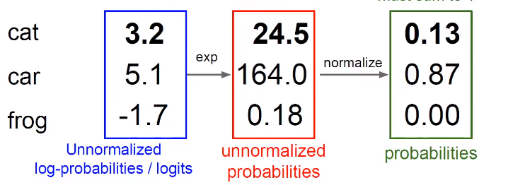
softmax把分数变成了概率，softmax不需要权重，本质进行了数学的运算。

\[\text{Softmax }P(Y=k|X=x_i)=\frac{e^{s_k}}{\sum_j e_{s_k}} \]

然后再构造交叉熵损失函数，表示混乱程度，或者叫对数似然损失函数(details in CS229)

$$ L_i=-logP(Y=k|X=x_i) $$ 想要得到全部分类正确的概率就是把三个分类正确的概率乘起来，那么实际上就是在把各自的log加起来，这样做把一个非常小的概率转换成了一个比较好的值，我们希望对数的值最大化。

那么这个\(Loss\)表示为：

\[L_i=-log(\frac{e^{s_k}}{\sum_j e_{s_k}}) \]

作业难点

def svm_loss_naive(W, X, y, reg):
    """
    Structured SVM loss function, naive implementation (with loops).

    Inputs have dimension D, there are C classes, and we operate on minibatches
    of N examples.

    Inputs:
    - W: A numpy array of shape (D, C) containing weights.
    - X: A numpy array of shape (N, D) containing a minibatch of data.
    - y: A numpy array of shape (N,) containing training labels; y[i] = c means
      that X[i] has label c, where 0 <= c < C.
    - reg: (float) regularization strength

    Returns a tuple of:
    - loss as single float
    - gradient with respect to weights W; an array of same shape as W
    """
    dW = np.zeros(W.shape)  # initialize the gradient as zero

    # compute the loss   and the gradient
    num_classes = W.shape[1]  # 这里shape[1]=10 shape[0]=3073 ,3073=32*32*3+1
    num_train = X.shape[0]  #  这里shape[0]=500 shape[1]=3073 相乘得到500*10
    loss = 0.0
    for i in range(num_train):  # 每次循环算一张图片
        scores = X[i].dot(W)
        correct_class_score = scores[y[i]]  # 这里y是单行的，即取出当前标签对应的值
        for j in range(num_classes):
            if j == y[i]:  # 这里的目的是不对自身相减 
                continue  # 比对每一个类别的偏差
            margin = scores[j] - correct_class_score + 1  # note delta = 1
            if margin > 0:
                loss += margin  #dW.shape ->(3073,10)
                dW[:, j] += X[i].T  # changed，这里是求梯度
                # 取第j列的元素以行形式返回
                dW[:, y[i]] -= X[i].T  # changed 

    # Right now the loss is a sum over all training examples, but we want it
    # to be an average instead so we divide by num_train.
    loss /= num_train
    dW /= num_train
    # Add regularization to the loss.
    loss += reg * np.sum(W * W)
    dW += 2 * reg * W
    #############################################################################
    # TODO:                                                                     #
    # Compute the gradient of the loss function and store it dW.                #
    # Rather than first computing the loss and then computing the derivative,   #
    # it may be simpler to compute the derivative at the same time that the     #
    # loss is being computed. As a result you may need to modify some of the    #
    # code above to compute the gradient.                                       #
    #############################################################################
    # *****START OF YOUR CODE (DO NOT DELETE/MODIFY THIS LINE)*****
    """check the code above"""
    # *****END OF YOUR CODE (DO NOT DELETE/MODIFY THIS LINE)*****

    return loss, dW

上面的求导是这样的：

\[\frac{\partial L_i}{\partial W_j}=\begin{cases} x_i^T(W_j-x_iW_i+\Delta >0)\newline 0(W_j-x_iW_i+\Delta <0) \end{cases} \]

\[\frac{\partial L_i}{\partial W_{Y_i}}=-x_i^T(W_j-x_iW_i+\Delta >0) \]

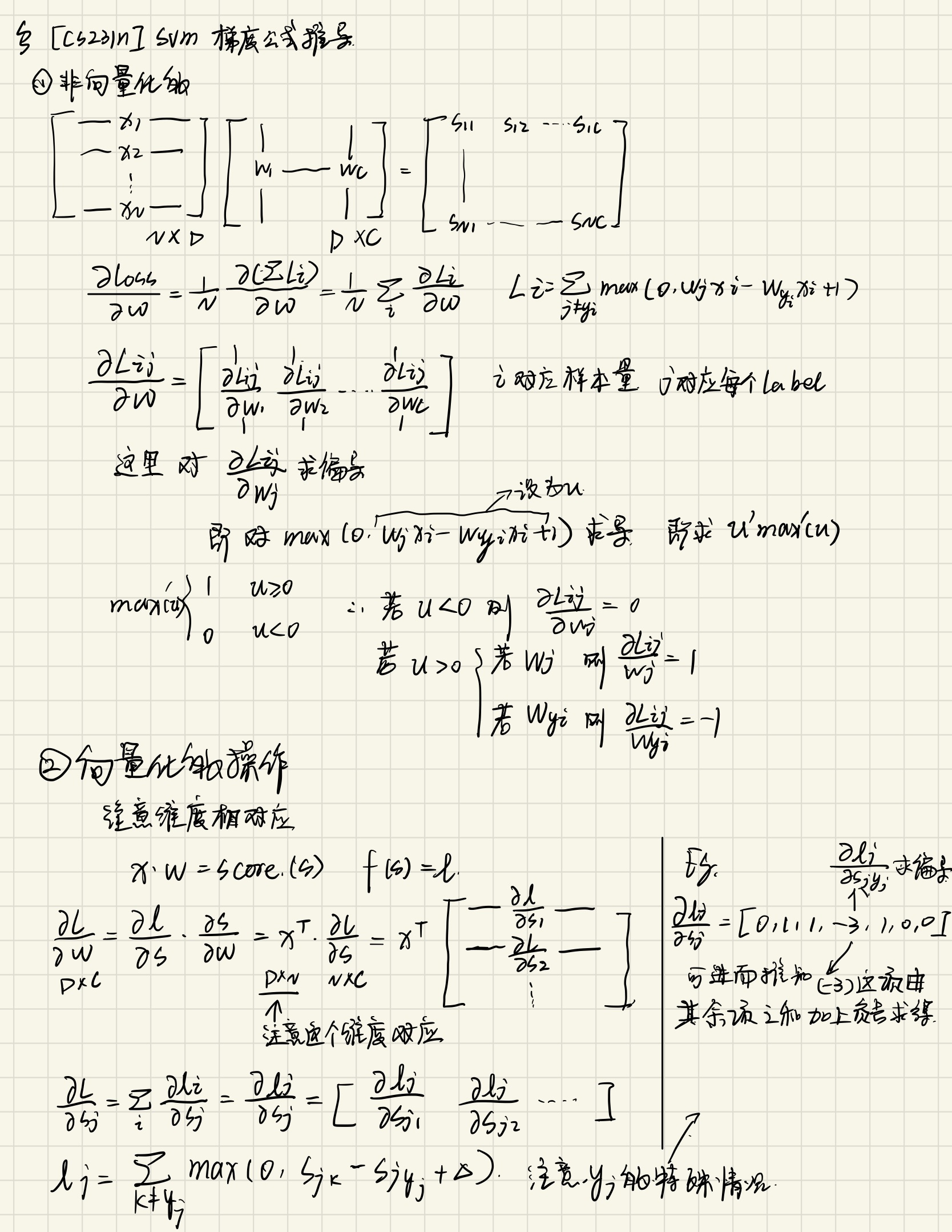
向量化的版本

d_score = (scores.T - correct_class_scores).T + 1
    d_score[d_score < 0] = 0  # max求导后的结果,下同
    d_score[d_score > 0] = 1
    d_score[np.arange(scores.shape[0]), y] = 0  # 清空原本就是同一类的值
    d_score[np.arange(scores.shape[0]), y] = -np.sum(d_score, axis=1)  # max在这里求导是-1
    dW = X.T @ d_score
    dW = dW / X.shape[0] + 2 * reg * W  # 求导后是两倍的

这里的减去x[i].T与-np.sum(d_score, axis=1)都是因为\(i=Y_i\) 情况下是score>0的，那么max求导后是-1