第三周作业:卷积神经网络
net = torch.nn.Sequential(
    Reshape(),
    nn.Conv2d(1, 6, kernel_size=5, padding=2), nn.Sigmoid(),
    nn.AvgPool2d(kernel_size=2, stride=2),
    nn.Conv2d(6, 16, kernel_size=5), nn.Sigmoid(),
    nn.AvgPool2d(kernel_size=2, stride=2),
    nn.Flatten(),
    nn.Linear(16 * 5 * 5, 120), nn.Sigmoid(),
    nn.Linear(120, 84), nn.Sigmoid(),
    nn.Linear(84, 10))

#对网络进行测试
X = torch.rand(size=(1, 1, 28, 28), dtype=torch.float32)
for layer in net:
    X = layer(X)
    print(layer.__class__.__name__,'output shape: \t',X.shape)
一:深度学习计算:
1.参数访问:net[ ].state_dict( )
net = nn.Sequential(nn.Linear(4,8), nn.ReLU(), nn.Linear(8, 1))

print(net[2].state_dict())

2.一次性访问所有参数: named_parameters()
print(*[(name, param.shape) for name, param in net[0].named_parameters()])
print(*[(name, param.shape) for name, param in net.named_parameters()])

3.内置初始化:
def init_normal(m):
    if type(m) == nn.Linear:
        #生成一个均值为0方差为1的权重
        nn.init.normal_(m.weight, mean=0, std=0.01)
        nn.init.zeros_(m.bias)
net.apply(init_normal)
net[0].weight.data[0], net[0].bias.data[0]
使用apply函数给net所有Linear层初始化
4.读写文件
存储张量:
#存储张量
x = torch.arange(4)
torch.save(x, 'x-file'
#读回内存
x2 = torch.load('x-file')
x2
加载和保存模型参数:
class MLP(nn.Module):
    def __init__(self):
        super().__init__()
        self.hidden = nn.Linear(20, 256)
        self.output = nn.Linear(256, 10)

    def forward(self, x):
        return self.output(F.relu(self.hidden(x)))

net = MLP()
X = torch.randn(size=(2, 20))
Y = net(X)

#将模型保存到mlp.params文件夹中
torch.save(net.state_dict(), 'mlp.params')

#模型恢复
clone = MLP()
clone.load_state_dict(torch.load('mlp.params'))
clone.eval()
二:卷积神经网络:
1.两个特性:
平移不变性:不管检测对象出现在图像中的哪个位置,神经网络的前面几层应该对相同的图像区域具有相似的反应
局部性(locality):神经网络的前面几层应该只探索输入图像中的局部区域,而不过度在意图像中相隔较远区域的关系。
2.目标边缘检测:
(1)构造一个6*8像素的黑白图像,中间为黑(0),其余为白(1)
X = torch.ones((6, 8))
X[:, 2:6] = 0
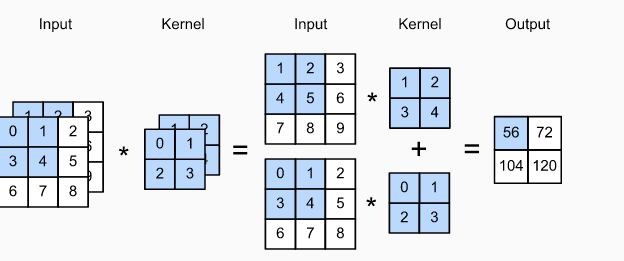
(2)构造一个卷积核,计算结果为相邻元素相同输出为0,否则为非0,然后计算。
#卷积核K
K=torch.tensor([[1.0],[-1.0]])
Y=corr2d(X,K)
Y
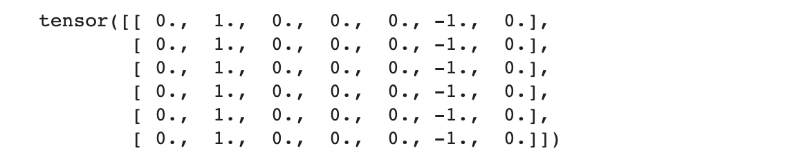
但这种方法只能检测垂直边缘,无法检测水平边缘。
# 构造一个二维卷积层,它具有1个输出通道和形状为(1,2)的卷积核
conv2d = nn.Conv2d(1,1, kernel_size=(1, 2), bias=False)

X = X.reshape((1, 1, 6, 8))
Y = Y.reshape((1, 1, 6, 7))

for i in range(10):
    Y_hat = conv2d(X)
    l = (Y_hat - Y) ** 2
    conv2d.zero_grad()
    l.sum().backward()
    conv2d.weight.data[:] -= 3e-2 * conv2d.weight.grad
    if (i + 1) % 2 == 0:
        print(f'batch {i+1}, loss {l.sum():.3f}')
conv2d.weight.data.reshape((1, 2))
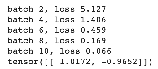
10轮迭代后,结果很接近我们预估的值。
3.填充和步幅
填充:如果我们添加 Ph行填充和 Pw 列填充,则输出形状将为:

填充的具体操作可以在nn.Conv2d中添加padding
步幅:当垂直步幅为 Sh 、水平步幅为 Sw时,输出形状为:

填充的具体操作可以在nn.Conv2d中添加stride
总结:
填充可以增加输出的高度和宽度。这常用来使输出与输入具有相同的高和宽。
步幅可以减小输出的高和宽,例如输出的高和宽仅为输入的高和宽的 1/𝑛1/n( 𝑛n 是一个大于 11 的整数)。
填充和步幅可用于有效地调整数据的维度。
4.多输入输出通道:
(1)多输入通道:
想关计算:
(2)多输出通道:
我们可以将每个通道看作是对不同特征的响应,因为每个通道不是独立学习的,而是为了共同使用而优化的。因此,多输出通道并不仅是学习多个单通道的检测器。
(3)1*1卷积:
可以改变通道数,可以加入非线形。
5.池化层:
(1).常用的方法有两种:最大值池化和平均值池化
(2)可以对池化层的步幅和填充进行调整:
#参数分别是池化窗口大小,填充大小和步幅大小
pool2d = nn.MaxPool2d((2, 3), padding=(1, 1), stride=(2, 3))
pool2d(X)
(3)在处理多通道输入数据时,池化层对每个通道进行单独运算,并非像卷积层一样在通道上对输入进行汇总,即:池化层的输出通道数和输入通道数相同。
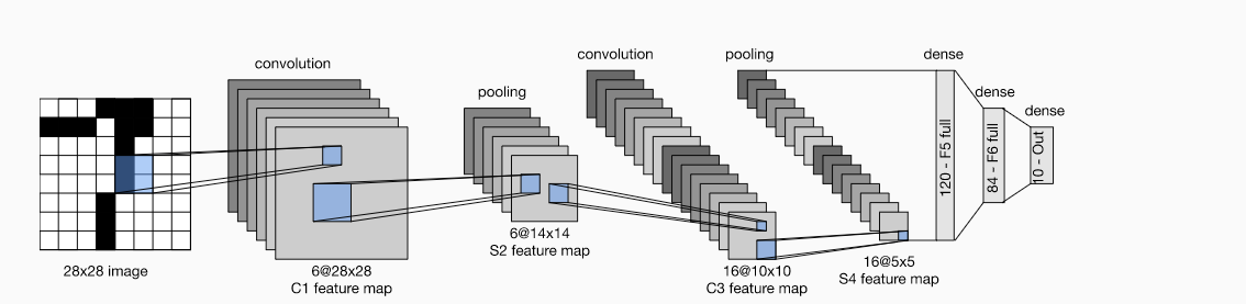
6.LeNet:
(1).大体结构:
(2)模型实现:
定义网络:
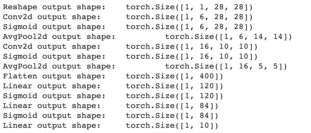
class Reshape(torch.nn.Module):
    def forward(self, x):
        return x.view(-1, 1, 28, 28)

net = torch.nn.Sequential(
    Reshape(),
    nn.Conv2d(1, 6, kernel_size=5, padding=2), nn.Sigmoid(),
    nn.AvgPool2d(kernel_size=2, stride=2),
    nn.Conv2d(6, 16, kernel_size=5), nn.Sigmoid(),
    nn.AvgPool2d(kernel_size=2, stride=2),
    nn.Flatten(),
    nn.Linear(16 * 5 * 5, 120), nn.Sigmoid(),
    nn.Linear(120, 84), nn.Sigmoid(),
    nn.Linear(84, 10))
对网络进行测试:
X = torch.rand(size=(1, 1, 28, 28), dtype=torch.float32)
for layer in net:
    X = layer(X)
    print(layer.__class__.__name__,'output shape: \t',X.shape)
使用Fashion-MNIST数据集进行训练:
batch_size = 256
train_iter, test_iter = d2l.load_data_fashion_mnist(batch_size=batch_size)

def evaluate_accuracy_gpu(net, data_iter, device=None): #@save
    if isinstance(net, torch.nn.Module):
        net.eval()
        if not device:
            device = next(iter(net.parameters())).device
    # 正确预测的数量,总预测的数量
    metric = d2l.Accumulator(2)
    for X, y in data_iter:
        if isinstance(X, list):
            X = [x.to(device) for x in X]
        else:
            X = X.to(device)
        y = y.to(device)
        metric.add(d2l.accuracy(net(X), y), y.numel())
    return metric[0] / metric[1]
#@save
def train_ch6(net, train_iter, test_iter, num_epochs, lr, device):
    def init_weights(m):
        if type(m) == nn.Linear or type(m) == nn.Conv2d:
            nn.init.xavier_uniform_(m.weight)
    net.apply(init_weights)
    print('training on', device)
    net.to(device)
    optimizer = torch.optim.SGD(net.parameters(), lr=lr)
    loss = nn.CrossEntropyLoss()
    animator = d2l.Animator(xlabel='epoch', xlim=[1, num_epochs],
                            legend=['train loss', 'train acc', 'test acc'])
    timer, num_batches = d2l.Timer(), len(train_iter)
    for epoch in range(num_epochs):
        metric = d2l.Accumulator(3)
        net.train()
        for i, (X, y) in enumerate(train_iter):
            timer.start()
            optimizer.zero_grad()
            X, y = X.to(device), y.to(device)
            y_hat = net(X)
            l = loss(y_hat, y)
            l.backward()
            optimizer.step()
            with torch.no_grad():
                metric.add(l * X.shape[0], d2l.accuracy(y_hat, y), X.shape[0])
            timer.stop()
            train_l = metric[0] / metric[2]
            train_acc = metric[1] / metric[2]
            if (i + 1) % (num_batches // 5) == 0 or i == num_batches - 1:
                animator.add(epoch + (i + 1) / num_batches,
                             (train_l, train_acc, None))
        test_acc = evaluate_accuracy_gpu(net, test_iter)
        animator.add(epoch + 1, (None, None, test_acc))
    print(f'loss {train_l:.3f}, train acc {train_acc:.3f}, '
          f'test acc {test_acc:.3f}')
    print(f'{metric[2] * num_epochs / timer.sum():.1f} examples/sec '
          f'on {str(device)}')
lr, num_epochs = 0.9, 10
train_ch6(net, train_iter, test_iter, num_epochs, lr, d2l.try_gpu())
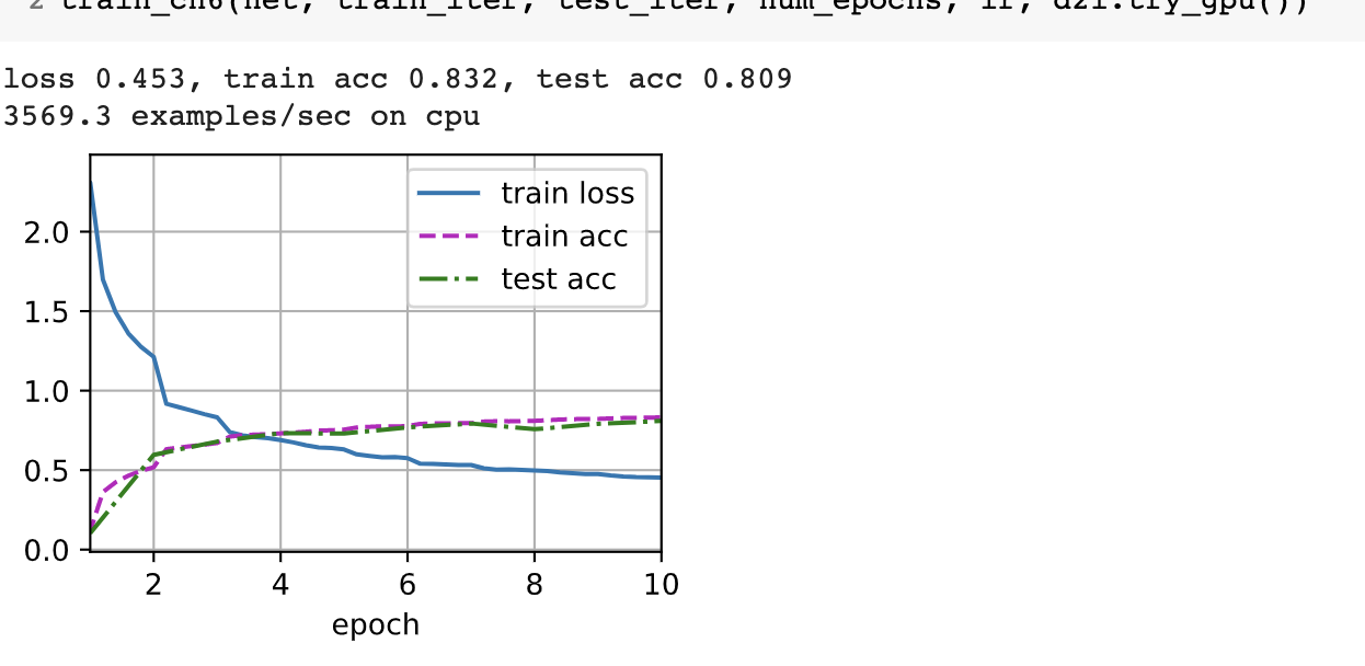
训练结果还可以
三.猫狗大战:
1.导入数据:
!wget http://fenggao-image.stor.sinaapp.com/dogscats.zip
!unzip dogscats.zip

!wget https://static.leiphone.com/cat_dog.rar
!unrar x /content/cat_dog.rar
2.定义网络:
import torch.nn.functional as F
import torch.optim as optim
class Net(nn.Module):
    def __init__(self):
        super(Net, self).__init__()
        self.conv1 = nn.Conv2d(3, 6, 5)
        self.pool = nn.MaxPool2d(2, 2)
        self.conv2 = nn.Conv2d(6, 16, 5)
        self.fc1 = nn.Linear(44944, 120)
        self.fc2 = nn.Linear(120, 84)
        self.fc3 = nn.Linear(84, 2)

    def forward(self, x):
        x = self.pool(F.relu(self.conv1(x)))
        x = self.pool(F.relu(self.conv2(x)))
        x = x.view(-1, 44944)
        x = F.relu(self.fc1(x))
        x = F.relu(self.fc2(x))
        x = self.fc3(x)
        return x

# 网络放到GPU上
net = Net().to(device)
criterion = nn.CrossEntropyLoss()
optimizer = optim.Adam(net.parameters(), lr=0.001)
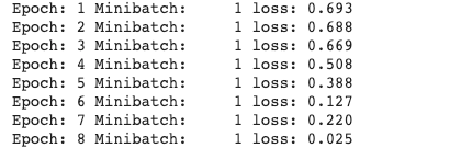
3.训练:
for epoch in range(10):  # 重复多轮训练
    for i, (inputs, labels) in enumerate(loader_train):
        inputs = inputs.to(device)
        labels = labels.to(device)
        # 优化器梯度归零
        optimizer.zero_grad()
        # 正向传播 + 反向传播 + 优化
        outputs = net(inputs)
        loss = criterion(outputs, labels)
        loss.backward()
        optimizer.step()
        # 输出统计信息
        if i % 100 == 0:
            print('Epoch: %d Minibatch: %5d loss: %.3f' %(epoch + 1, i + 1, loss.item()))

print('Finished Training')
4.在比赛用的测试集上进行测试:
loader_test = torch.utils.data.DataLoader(dsets, batch_size=1, shuffle=False, num_workers=0)

def test(model,dataloader,size):
    model.eval()
    cnt = 0    #count
    for inputs,_ in dataloader:
      if cnt < size:
        inputs = inputs.to(device)
        outputs = model(inputs)
        _,preds = torch.max(outputs.data,1)
        key = dsets.imgs[cnt][0].split("/")[-1].split('.')[0]
        final[key] = preds[0]
        cnt += 1
      else:
        break;
    print('Accuracy of the network on the 10000 test images: %d %%' % (
    100 * correct / total))
test(net,loader_test,size=2000)
5.保存数据:
with open("/content/test.csv",'a+') as f:
    for key in range(2000):
        f.write("{},{}\n".format(key,final[str(key)]))
6.上交结果:


训练了两次,结果相差不多,但都并非很理想。
复习使用了VGGNET进行了一次训练:


 浙公网安备 33010602011771号